Munich Personal RePEc Archive
The Demand for Current Public
Expenditure in Fiji: Theory and
Empirical Results
Doessel, Darrel and Valadkhani, Abbas
Queensland Centre for Schizophrenia Research, UNE Business
School, University of New England
2003
Online at
https://mpra.ub.uni-muenchen.de/50392/
THE DEMAND FOR CURRENT PUBLIC EXPENDITURE IN FIJI:
THEORY AND EMPIRICAL RESULTS
By
D.P. DOESSEL
Queensland Centre for Schizophrenia Research The Park-Centre for Mental Health
Cnr Ellerton Drive and Walston Park Road Wacol QLD 4076
Tel: +61-7- 3271 8805 (W) and +61-7-3378 6853 (h) Fax: +61-7-3271 8698
and
ABBAS VALADKHANI Lecturer
School of Economics and Finance Queensland University of Technology
GPO Box 2434
Brisbane, Qld 4001, Australia. Email: a.valadkhani@qut.edu.au
Tel: +61-7-3864 1233 Fax: +61-7-3864 1500 (All correspondence to Dr Valadkhani)
Biographical details:
1) D.P. Doessel was a Reader in Economics at The University of Queensland. He is now undertaking full-time research at the Queensland Centre for Schizophrenia Research.
The demand for current public expenditure in Fiji: theory and empirical
results
*Abstract
This paper analyses current government expenditure in Fiji using annual time series data for
the period 1969-1999. Alternative theories of government expenditure are reviewed and a
distinction is made between economic/apolitical determinants and institutional/political
determinants. Categorising the literature in this way suggests the application of non-nested
tests in empirical work, which is reported elsewhere. All non-nested tests lead to the
conclusion of double rejection. Therefore, a parsimonious comprehensive model,
encompassing both economic and institutional variables, is preferred as it passes all
diagnostic tests and exhibits no sign of misspecification. The Engle-Granger two-step
procedure has been applied to analyse both long- and short-run determinants of public
expenditure. The paper presents the first empirical estimates of the own-price elasticity of
demand and income elasticity of demand for current public expenditure in Fiji.
Introduction
Fiji became independent in 1970 with Ratu Sir Kamisese Mara as Prime Minister after nearly
a century as a British colony. Fiji had a population of 801000 in 1999 and has been classified
as a lower middle income country by the World Bank, with a per capita annual income of
US$2310 (World Bank, 2001). Although it is one of the most developed of the Pacific island
economies, it still has a large subsistence sector and the economy can be regarded as
dualistic. Sugar and clothing are the main (commodity) export industries. Political
uncertainties have created economic uncertainties. Coups in 1987 and more recently in May
*We wish to acknowledge the helpful comments of two anonymous referees. The usual caveat
2000 have created an economic environment which is not conducive to long-term investment
as a result of poorly-defined property rights and migration of skilled workers (Gani, 1998).
For an account of recent economic events see Chand (1998) and for political and
constitutional events see Lal and Lamour (1997).
Given this turbulent recent history concerning governance it is relevant to apply
contemporary public finance theories on the determinants of the size of the government
sector. The objective of this paper is to do just that.
Since the pioneering studies by Borcherding and Deacon (1972) and Bergstrom and
Goodman (1973) the analysis of the size of the government sector has ceased to be
characterised by the atheoretical or ad hoc analyses that were dominant until then. For
bibliographies of the early literature see Pryor (1968: 46-51) and Borcherding (1977: 67-70).
Essentially the modern analysis of the demand for goods and services provided by
government involves an application of the median voter hypothesis, associated with Downs
(1957). This conception will be referred to below as ‘the economic/apolitical model’.
In essence the demand for public goods is conceived of as the outcome of the demand
for public goods by the median voter, or as Borcherding (1985) puts it, by “the Fiscal
Everyman”. Put otherwise, the demand for government expenditure is to be seen as a
function of the characteristics of the median voter. This conceptual framework leads to a
relatively parsimonious specification of the explanatory variables in the demand equation.
Those factors are as follows: prices, income and population, as well as some other relevant
variables. For an exposition see, inter alia, Larkey, Stolp and Winer (1981), Mueller (1989)
and Brown and Jackson (1986).
This conceptual framework is, by no means, the only theory of government
expenditure. For instance, Wagner (1883) had argued that the public sector expands as the
(1967) have argued that government expenditure is subject to a “displacement effect”
associated with some crisis such as war; and Nordhaus (1975) has argued that government
expenditure (and other macroeconomic variables) are subject to “political business cycles”.
It is not our purpose here to enumerate these numerous theories and/or create a new
classification scheme. See for example Lybeck (1986) for a 12-fold classification of such
theories, Henrekson (1988) for a categorisation of demand and supply side determinants and
Mueller (1989: 320-47) for a five-fold classification scheme.
The approach adopted in this paper is to categorise explanatory variables of
government expenditure as being of an economic/apolitical kind or of an
institutional/political nature. This dual scheme has been employed by Borcherding (1985)
and Halsey and Borcherding (1997). Such a formulation suggests a means by which an
indication of the relative importance of these two models can be established. Viewing
explanatory variables in this way invites the application of non-nested econometric tests.
A second important approach to explain government expenditure is what is referred to
below as “the institutional model”. This approach covers a wide range of issues such as the
political business cycle (Rogoff, 1990), political unrest/revolt (such as the coups of
1987-1988 and 2000), macroeconomic variables such as unemployment and inflation, the power of
pressure groups (Tullock, 1959, Stigler, 1970, Olson, 1982, Mueller and Murrell, 1986, and
Marlow and Orzechowski, 1996), fiscal illusion (Buchanan, 1967), and incrementalism
(Wildavsky, 1964). Also, it should be recognised that exogenous shocks, such as the oil
embargo of 1973 and 1974, can have important repercussions on government expenditure.
The structure of this paper is as follows: The next section presents a theoretical
framework for the analysis. The following section provides a brief account of the structure of
the government sector in Fiji and some relevant time series data on the phenomena to be
econometric results of the Engle-Granger two-step procedure. Some concluding remarks will
be presented in the final section.
Theoretical framework and estimation procedure
It is not our purpose here to provide a comprehensive review and evaluation of the theoretical
and empirical literature on the demand for public goods: such a review is provided recently in
Doessel and Valadkhani (2002). We provide here only a brief outline of the framework of the
estimating procedure we have adopted.
The economic/structural model
Following Gemmell (1990), the demand for real government expenditure can be stated as
follows:
(
)
Gt = A P P Y POP POP gtβ1 ytβ2 t / t β3 βt4
(1)
where Gt is real government consumption expenditure,
A is a constant,
Pgt is the price of government-provided goods and services, as measured by the
government price deflator,
Pyt is the price of private goods and services as measured by the GDP deflator,
Yt is real GDP,
POPt is population, and
1, 2, 3 and 4 are elasticities to be estimated.
This equation bears a close resemblance to the formulations in Borcherding and
Deacon (1972) and Bergstrom and Goodman (1973). For details see Gemmell (1990). Our
2
0 1 3 4
5 ( ) 1
ln( ) ln( / ) ln( / ) ln( ) ln( )
gt yt t t
t t t
t t
DV coup
G β β P P β Y POP β POP β AGEMR
β ε
= + + + + +
+ (2)
where AGEMR is the ratio of agricultural employment to total employment, DV(Coup) is an
intercept dummy variable which takes the value of 1 for the coups of the 1987-1988
period, and zero otherwise, and
ε
1 is a well-behaved error term.A brief explanation for the inclusion of these explanatory variables was in the previous
section.
The institutional model
An important advance in the study of the public sector occurred in the 1950s, when some
economists applied the tools of their trade to non-market decision making, i.e. economic
theory was applied to issues which had previously been in the domain of political science.
This development, initiated by, inter alia, Black (1948), Downs (1957), and Buchanan and
Tullock (1962), is now generally referred to as "public choice". See Mueller (1989) for a
comprehensive account of this approach.
An important conclusion from the public choice school is that the outcomes of the
public sector are determined, in part, by institutions, their procedures and the people working
in those institutions. In other words, fiscal institutions can determine outcomes. This
seemingly trite point, i.e. that institutions matter, is central to the public choice literature. As
Buchanan and Wagner (1977: 636) put it "We are institutionalists in the sense that we think
that arrangements or rules do affect outcomes."
The institutional model we are estimating can be specified as follows:
0 1 2 3 4
5 6 7 8 2
ln( ) ln( ) ln( ) ln( )
ln( ) ln( ) ln( ) ( )
t t t t t
t t yt t
G EDV U SEREMR OPEN
HHIT DTAXR P DV coup
α α α α α
α α α α ε
= + + + + +
+ + ∆ + + (3)
where EDV is an intercept dummy variable which equals unity when there has been an
SEREMR is the ratio of service employment to total employment,
OPEN is an index of openness as defined by total exports and imports divided by
GDP,
U is the rate of unemployment,
HHIT is the Hirschman-Herfindahl index (Hirschman, 1964) of tax complexity,
DTAXR is the ratio of direct taxes to total taxes, and
ln(Py) is the inflation rate using the GDP price deflator.
A rationale for these explanatory variables was considered briefly in the introductory
section. For a more detailed account of the literature on the theoretical underpinning of these
explanatory variables see Doessel and Valadkhani (2002). Table 1 summarises both the
notation to be employed in this study and the expected theoretical signs of the relevant
explanatory coefficients in both the economic/structural model and the institutional model.
[Table 1 about here]
Estimation procedure
The empirical procedure has been to estimate equation (2) and equation (3)
separately. These two equations performed quiet well in terms of goodness-of-fit, most of the
coefficients being statistically significant (at the 5 per cent level), and having the expected
theoretical signs. However, there were some diagnostic tests which indicated misspecification
in the institutional model and serious autocorrelation in the economic model. Furthermore,
the application of non-nested tests [the Cox test, the Ericsson Instrumental Variable (IV) test,
the Sargan restricted/unrestricted reduced form test, and the encompassing (F) test, Hendry
and Doornik (1999)], to these separate models explaining government expenditure, indicate
rejection of each model. Essentially these results signify that an explanation of government
economic/apolitical model. These non-nested test results and estimated equations (2) and (3),
not reported here, have been published elsewhere (Doessel and Valadkhani, 2002). Therefore,
attention is now directed to the specification and estimation of a comprehensive model
including all the variables in both models. We have applied general-to-specific econometric
methodology to estimate the following comprehensive model, which captures the long-run
determinants of public expenditure:
0
6 7 8 9
10 11 12
2
1 3 4
5
ln( ) ln( / ) ln( / ) ln( ) ln( )
( ) ln( ) ln( ) ln( )
ln( ) ln( ) ln( )
t gt yt t t t t
t t t t t
t t yt t
G P P Y POP POP AGEMR
DV coup EDV U SEREMR OPEN
HHIT DTAXR P e
λ λ λ λ λ
λ λ λ λ λ
λ λ λ
= + + + + +
+ + + + +
+ + ∆ +
(4)
An important step before estimating equation (4) is to determine the time series
properties of the data. This is an important issue since the use of non-stationary data in the
absence of cointegration can result in spurious regression results. To this end, the Augmented
Dickey-Fuller (ADF) test has been adopted to examine the stationarity, or otherwise, of the
time series data. It was found that all the time series variables in equation (4) were I(1), or
stationary after first differencing. In this paper the lowest value of the Akaike Information
Criterion (AIC) has been used as a guide to determine the optimal lag length in the ADF
regression. These lags are added to the ADF regression to ensure that the error term is white
noise. It is worth emphasising that since there are only 31 annual observations for the various
variables studied in this paper, the unit root test results should be taken with a pinch of salt as
the ADF test is appropriate for large samples.
Let us assume that all the variables in equation (4) are I(1) and the resulting residuals
are I(0). According to Engle and Granger (1987), it can then be stated that there exists a
( )
( ) ( )( )
0 1 2 3 4
5 6 7 8
0 0 0 0
0 0 0 0
ln ln ln ln ln
ln ln( ) ln( ) ln( )
t i i i i
i i i i
p p p p
g
t i t i
i p t i i t i i i
p p p p
t i t i t i
t i
i i i i
P Y
POP
P POP
SEREMR OPEN HHIT
G AGEMR
U
γ γ γ γ γ
γ γ γ γ
− − = − = − = = − − − − = = = = ∆ = + ∆ + ∆ + ∆ ∆ + ∆ ∆ + ∆ ∆ + + + ( ) 9 10 2
11 12 1
0 0 1
ln( ) ln( ) ln
i i ( ) i t
p p p
t i yt t i t i t
i i i
t t e
DTAXR P DV coup EDV G θ ν
γ − γ − γ γ δ − −
= = =
+
+ ∆ + ∆ + + + ∆ +
(5)
where
γ
ji are the estimated short-term coefficients;θ
represents the feedback effect or thespeed of adjustment whereby short-term dynamics converge to the long-term equilibrium
path formulated in equation (4);
δ
i denotes the estimated coefficients of the lagged dependentvariable to ensure that vt or the disturbance term is white noise; e, or the ECM, is obtained
from equation (4), and ∆ indicates the first-difference operator.
The general-to-specific methodology can be used to omit insignificant variables in
equation (5) on the basis of a battery of maximum likelihood tests. In this method, joint zero
restrictions are imposed on explanatory variables in the unrestricted (general) model to obtain
the most parsimonious and robust equation in the estimation process. However, one may
argue that the Engle-Granger method is appropriate if there are only two variables in the
cointegrating equation. In other words, if there are more than two variables, it is possible that
there could exist more than one cointegrating relationship between the variables, rendering
the Engle-Granger two step procedure inadequate. To address this issue the multivariate
Johansen cointegration technique was initially used to determine the number of cointegrating
vectors. However, given the lack of long and consistent time series data (i.e only 31
observations), the Johansen method is also inappropriate, as the cointegration results, with
only 31 observations, were very sensitive to the lag length, the inclusion or exclusion of the
intercept term, or a trend in the cointegration equation, and/or the VAR specification. It
should be noted that the max-eigenvalue and trace tests on equation (4) indicate that there is
one cointegrating vector at the 1 per cent level. In these tests we have allowed only one lag
vector and the VAR model. The multivariate cointegration test results have not been reported
here but they are available from the authors upon request.
Some relevant time series data on government in Fiji
As mentioned previously Fiji is categorised as a lower middle income country by the World
Bank. Unlike federations such as the US, Canada, Australia and Germany, Fiji has a
government structure which consists of only a central government and a (relatively small)
local government sector. In this respect it is similar to the United Kingdom (pre-devolution)
and New Zealand.
This study employs aggregate data on all public expenditure. It would be desirable if
we could separate government expenditure (say) on the security system and defence, given
that governments may make decisions on defence expenditure in a quiet different way from
civilian expenditure. However, such a disaggregation of the data is not available for the
1969-1999 period. This creates an apples-and-oranges problem which we cannot resolve. Data
limitations preclude a disaggregated analysis.
Figure 1 presents time series data on real GDP and real government current
expenditure (in 1989 constant prices) for the period analysed in this study, 1969-1999. It is
clear that GDP has experienced some fluctuations through time. Note the decrease in GDP
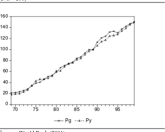
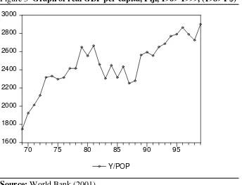
and government expenditure in 1987 and 1988. Figure 2 shows the plot of government and
GDP deflators whereas Figure 3 presents a graph of real GDP per capita. As can be seen the
impact of the 1987-1988 military coups on real GDP per capita is quiet evident. For further
details on the structure of the Fiji economy see, inter alia, Kasper, Bennett and Blandy (1988)
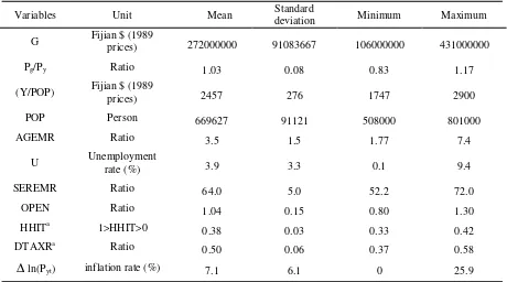
and Treadgold (1992). Table 2 presents descriptions of the data employed and summary
statistics.
[Table 2 about here]
Empirical results and policy implication of study
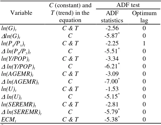
As mentioned above it is very important to examine the time series properties of the data. The
empirical results of the ADF unit root test are summarised in Table 3. According to the test
results, all of the variables appearing in the estimated parsimonious equation reported in
Table 4 are integrated of order one, I(1), and they become stationary after first differencing.
Since all the variables in equation (4) are I(1), the Engle-Granger two-step procedure can be
used to examine if this equation represents a long-term relationship.
[Table 3 about here]
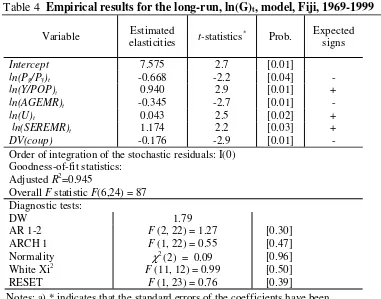
Table 4 presents the results of estimating the comprehensive long-run model of public
expenditure in Fiji using the 1969-1999 data. As seen, all the estimated coefficients are
significant at least at the 5 per cent level and have the expected theoretical signs. This
equation performs very well in terms of goodness-of-fit (adjusted R2 = 0.945) and passes the
overall F test at the one per cent level. In addition, this equation passes each and every
diagnostic tests.
[Table 4 about here]
There are a number of important points that can be drawn from the estimated long-run
coefficients of the public expenditure model. First, the relative price coefficient (–0.67)
indicates that the demand for government goods and services in Fiji is inelastic. This
coefficient is in the relevant range reported in the prior literature. Second, the coefficient on
per capita income (+0.94) indicates that the demand for public goods and services is normal:
given that this coefficient is less than unity, there is no evidence that Wagner’s law applies in
the context of Fiji. Third, this comprehensive model includes the measure of structural
means that in the long-run as the agricultural sector of the Fijian economy declines in relative
importance, there is an increased demand for existing services, and/or a demand for new
services, provided by government.
Fourth, the variable (SEREMR), measuring interest group influence, is highly
significant with a relatively larger long-run elasticity of 1.17. This is not counter-intuitive
given the nature of government decision-making processes in Fiji. Borcherding’s (1985)
inability to specify the numerical importance of the institutional variables did not indicate
that such variables were irrelevant: this econometric analysis shows conclusively that
“institutions matter” in terms of explaining the growth of recurrent government expenditure
in Fiji. Fifth, it is also important to observe that the 1987-1988 military coups, as measured
by DV(Coup), have exerted a highly significant adverse impact on government expenditure
in Fiji.
As mentioned earlier, insignificant variables, the taxation variables concerning fiscal
illusion (i.e. HHIT, and DTAXR), EDV, OPEN and inflation, were omitted by applying
several maximum likelihood tests involving joint restrictions on explanatory variables in
order to obtain the most parsimonious and robust estimates. Also we have undertaken
exhaustive diagnostic tests. (The estimated results have been obtained by using PcGive 9.21
(Hendry and Doornik, 1999).
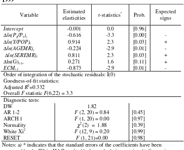
Attention is now directed to the second stage of the Engle-Granger representation
procedure. Table 5 presents the estimated results of an error correction model (ECM)
capturing short-run dynamics of public expenditure as formulated in equation (5). The
general-to-specific methodology has been adopted in estimating equation (5) by omitting
insignificant lagged variables and undertaking a battery of maximum likelihood tests. Joint
zero restrictions have been imposed on insignificant explanatory variables in the unrestricted
process. The parsimonious short-term model of public expenditure includes all of the
long-term delong-terminants of public expenditure except for U and DV(Coup).
[Table 5 about here]
In other words, the results reported in Table 5 indicate that the short-run sources of
the growth of public expenditure are changes in relative prices, per capita income, the ratio of
agriculture employment to total employment, the ratio of service employment to total
employment; and the lagged growth rate of public current expenditure. All the estimated
coefficients are statistically significant at least at the 5 per cent level, with the only exception
being
∆
ln(G)t-1, and have the expected signs. Having the expected sign with a magnitude of0.27, the variable
∆
ln(G)t-1 is a proxy to capture bureaucratic inertia or incrementalism. Thisvariable is statistically significant at the 11 per cent level. In terms of goodness-of-fit
statistics, though expressed in
∆
ln, with an adjusted R2 of 0.332, the short-run dynamicequation performs reasonably well. As with equation (4), this equation also passes each and
every diagnostic test. Table 5 also reveals that the feed-back coefficient (or adjustment speed)
is as high as –0.873, indicating that in every year 87 per cent of the divergence between the
short-run public expenditure growth from its long-run path, as formulated in equation (4), is
eliminated.
The significance of this paper lies in the fact that it presents the first empirical
estimates of the magnitudes of those factors that can explain current government expenditure
in Fiji. Thus policy makers (and their bureaucrats) now have a means whereby they can
predict the effect on government expenditure of changes in important determining variables
of that expenditure. Hence, one of the “black holes” that had previously confronted Fiji’s
Concluding Remarks
The existing literature of the demand for government goods and services is dominated by
studies of western countries and services provided by state or local governments. This study
is “a little bit different” in that it is one of the first such studies of a middle income country,
with a (single) government sector providing services generally supplied by central and state
governments in other countries. With respect to the first point it should not be automatically
concluded that economic analysis of this kind is not applicable to a country such as Fiji: it
should be recalled that Pryor (1968) succeeded in analysing government behaviour of
countries with markedly different systems, and that Wagner and Weber (1975) successfully
analysed governments with different organisational and behavioural (competition or
monopoly) characteristics.
The central focus of this paper is to provide an answer to the question posed by
Borcherding (1985) concerning the relative importance of long- and short-run
economic/apolitical and institutional/political factors in determining government expenditure
in Fiji. It is found that variables from both the institutional/political model and the
economic/apolitical model of the determinants of the demand for government services are
necessary. Thus, this study provides, not only further evidence that “institutions matter”, but
that the conventional economic variables are also necessary to explain current government
Table 1 Economic/structural and institutional explanatory variables applied in the real demand for government expenditure in Fiji
Variable name Variable definition Expected sign
Economic/Apolitical
Pg Government price deflator –
Py GDP price deflator +
Pg/Py Relative price ratio –
Y/POP Real per capita GDP +
POP Population zero or +
AGEMR Ratio of agricultural employment to total
employment –
Institutional/Political
Gt-1 or ∆Gt-1 Lagged real government expenditure (bureaucratic
inertia or incrementalism) + SEREMR Ratio of service employment to total employment +
OPEN Index of openness defined as total exports plus imports, divided by GDP -
∆ln(Pyt) Inflation rate using GDP price deflator +
U Unemployment rate +
HHIT Hirschman-Herfindahl index of tax complexity – DTAXR Ratio of direct taxes to total taxes –
EDV Election dummy variable +
Figure 1 GDP and real government consumption expenditure (G), Fiji, 1969-1999, F$ million (1989 prices)
500 1000 1500 2000 2500
100 200 300 400 500
70 75 80 85 90 95
GDP G
coups
GDP G
Source: World Bank (2001).
[image:17.595.75.412.468.738.2]Note: The left-hand scale indicates GDP (F$ million) and the right-hand scale measures government current expenditure (F$ million), both in constant 1989 prices.
Figure 2 Plot of government and GDP deflators, Fiji, 1969-1999,
(1989=100)
0 20 40 60 80 100 120 140 160
70 75 80 85 90 95
Pg Py
Figure 3 Graph of real GDP per capita, Fiji, 1969-1999, (1989 F$)
1600 1800 2000 2200 2400 2600 2800 3000
70 75 80 85 90 95
Y/POP
Table 2 Summary statistics and description of the data employed, Fiji, 1969-1999
Variables Unit Mean Standard
deviation Minimum Maximum
G Fijian $ (1989
prices) 272000000 91083667 106000000 431000000 Pg/Py Ratio 1.03 0.08 0.83 1.17
(Y/POP) Fijian $ (1989
prices) 2457 276 1747 2900
POP Person 669627 91121 508000 801000
AGEMR Ratio 3.5 1.5 1.77 7.4
U Unemployment
rate (%) 3.9 3.3 0.1 9.4
SEREMR Ratio 64.0 5.0 52.2 72.0
OPEN Ratio 1.04 0.15 0.80 1.30
HHITa 1>HHIT>0 0.38 0.03 0.33 0.42
DTAXRa Ratio 0.50 0.06 0.37 0.58
∆ln(Pyt) inflation rate (%) 7.1 6.1 0 25.9
Sources: World Bank (2001), Asian Development Bank (1995), International Monetary Fund (various) and International Labour Office (various).
Table 3 ADF test results of the data employed in
Tables 4 and 5, Fiji
Variable
C (constant) and T (trend) in the
equation
ADF test ADF
statistics
Optimum lag
ln(G)t C & T -2.56 0
∆ln(G)t C -5.87
*
0 ln(Pg/Py)t C & T -2.25 1
∆ ln(Pg/Py)t C -5.51
*
0 ln(Y/POP)t C & T -3.34 0
∆ ln(Y/POP)t C -6.21
*
0 ln(AGEMR)t C & T -3.09 0
∆ ln(AGEMR)t C -7.00
*
0
ln(U)t C & T -1.53 0
∆ ln(U)t C -5.15
*
0 ln(SEREMR)t C & T -2.81 0
∆ ln(SEREMR)t C -5.79
*
0
ECMt C & T -5.38* 0
*
Table 4 Empirical results for the long-run, ln(G)t, model, Fiji, 1969-1999
Variable Estimated
elasticities t-statistics *
Prob. Expected signs
Intercept 7.575 2.7 [0.01]
ln(Pg/Py)t -0.668 -2.2 [0.04] -
ln(Y/POP)t 0.940 2.9 [0.01] +
ln(AGEMR)t -0.345 -2.7 [0.01] -
ln(U)t 0.043 2.5 [0.02] +
ln(SEREMR)t 1.174 2.2 [0.03] +
DV(coup) -0.176 -2.9 [0.01] -
Order of integration of the stochastic residuals: I(0) Goodness-of-fit statistics:
Adjusted R2=0.945
Overall F statistic F(6,24) = 87 Diagnostic tests:
DW 1.79
AR 1-2 F (2, 22) = 1.27 [0.30]
ARCH 1 F (1, 22) = 0.55 [0.47]
Normality χ2
(2) = 0.09 [0.96] White Xi2 F (11, 12) = 0.99 [0.50]
RESET F (1, 23) = 0.76 [0.39]
Notes: a) * indicates that the standard errors of the coefficients have been corrected by the White HAC method before calculating t-ratios; b) figures in square brackets show the corresponding probabilities; and c) the estimated method is OLS.
Table 5 Empirical results for the short-run, ∆∆∆∆ln(G)t, model, Fiji,
1971-1999
Variable Estimated
elasticities t-statistics *
Prob. Expected signs
Intercept -0.001 0.0 [0.96]
∆ln(Pg/Py)t -0.616 -3.3 [0.00] -
∆ln(Y/POP)t 0.914 2.3 [0.03] +
∆ln(AGEMR)t -0.224 -2.9 [0.01] -
∆ln(SEREMR)t 0.811 2.3 [0.03] +
∆ln(G)t-1, 0.271 1.6 [0.11] +
ECMt-1 -0.873 -2.9 [0.01] -
Order of integration of the stochastic residuals: I(0) Goodness-of-fit statistics:
Adjusted R2=0.332
Overall F statistic F(6,22) = 3.3 Diagnostic tests:
DW 1.82
AR 1-2 F (2, 20) = 0.84 [0.45]
ARCH 1 F (1, 20) = 0.00 [0.97]
Normality χ2
(2) = 1.88 [0.39]
White Xi2 F (12, 9) = 0.20 [0.99]
RESET F (1, 21)=0.00 [0.98]
References
Asian Development Bank, (various). Key Indicators of Developing Asian and Pacific
Countries, Oxford University Press, Singapore.
Bergstrom, T.C. and Goodman, R.P., 1973. ‘Private demands for public goods’, American
Economic Review, 63(3): 280-96.
Black, D., 1948. ‘On the rationale of group decision making’, Journal of Political Economy,
56(1): 23-24.
Borcherding, T.E. and Deacon, R.T., 1972. ‘The demand for the services of non-federal
governments’, American Economic Review, 62(5): 891-901.
Borcherding, T.E., 1977. ‘The sources of growth of public expenditures in the United States,
1902-1970’, in T.E. Borcherding, (ed) Budgets and Bureaucrats: The Sources of Government
Growth, Duke University Press, Durham: 45-70.
Borcherding, T.E., 1985. ‘The causes of government expenditure growth: a survey of the US
evidence’, Journal of Public Economics, 28(3): 359-82.
Brown, C.V. and Jackson, P.M. 1986. Public Sector Economics, 3rd edn, Basil Blackwell,
Oxford.
Buchanan, J.M., 1967. Public Finance in Democratic Process: Fiscal Institutions and
Individual Choice, The University of North Carolina Press, Chapel Hill.
Buchanan, J.M. and Tullock, G., 1962. The Calculus of Consent: Logical Foundations of
Constitutional Democracy, University of Michigan Press, Ann Arbor.
Buchanan, J.M. and Wagner, R.E., 1977. Democracy in Deficit: The Political Legacy of Lord
Keynes, Academic Press, New York.
Chand, S., 1998. ‘Current events in Fiji: an economy adrift in the Pacific’, Pacific Economic
Bulletin, 13(1): 1-17.
Doessel, D. P. and Valadkhani, A. (2002). ‘Public finance and the size of government: a
literature review and econometric results for Fiji’, Discussion Paper No. 108, School of
Economics and Finance, Queensland University of Technology, Brisbane.
Downs, A., 1957. An Economic Theory of Democracy, Harper and Row, New York.
Engle, R. F. and Granger, C.W.J. (1987). ‘Cointegration and error correction: representation,
estimation and testing’, Econometrica, 55: 251-76.
Gani, A., 1998. ‘Some empirical evidence on the determinants of immigration from Fiji to
Gemmell, N., 1990. ‘Wagner’s law, relative prices and the size of the public sector’, The Manchester School of Economic and Social Studies, 58(4): 361-77.
Halsey, C.M. and Borcherding, T.E., 1997. ‘Why does government’s share of national income grow? an assessment of the recent literature on the US experience’, in Mueller, D.C.
(ed), 1997, Perspectives on Public Choice: A Handbook, Cambridge University Press, New
York: 562-89.
Hendry, D.F. and Doornik, A., 1999. Empirical Econometric Modelling Using PcGive for
Windows, Timberlake Consulting, London.
Henrekson, M., 1988. ‘Swedish government growth: a disequilibrium analysis’, in J.A.
Lybeck and M. Henrekson (eds), Explaining the Growth of Government, North Holland,
Amsterdam: 231-63.
Hirschman, A.O., 1964. ‘The paternity of an index’, American Economic Review, 54(5):
761-62.
International Labour Office, (various). Yearbook of Labour Statistics, ILO, Geneva.
International Monetary Fund, (various). Government Financial Statistics, IMF, Washington
DC.
Kasper, W., Bennett, J. and Blandy, R., 1988. Fiji: Opportunity from Adversity, The Centre
for Independent Studies, Sydney.
Lal, B.V. and Larmour, P., 1997. (eds.), Electoral Systems in Divided Societies: The Fiji
Constitution Review, Pacific Policy Paper 21, National Centre for Development Studies, Canberra.
Larkey, P.D., Stolp, C. and Winer, M., 1981. ‘Theorising about the growth of government: a
research assessment’, Journal of Public Policy, 1: 157-220.
Lybeck, J.A., 1986. The Growth of the Government in Developed Countries, Gower,
Aldershot.
Marlow, M.L. and Orzechowski, M.L., 1996. ‘Public sector unions and public spending’,
Public Choice, 89(102): 1-16.
Mueller, D. and Murrell, P., 1986. ‘Interest groups and the size of government’, Public
Choice, 48(2): 125-45.
Mueller, D.C., 1989. Public Choice II, Cambridge University Press, New York.
Nordhaus, W., 1975. ‘The political business cycle’, Review of Economic Studies, 42(2):
169-190.
Olson, M., 1982. The Rise and Decline of Nations: Economic Growth, Stagflation and Social
Peacock, A.T. and Wiseman, J., 1967. The Growth of Public Expenditure in the United Kingdom, 2nd edn, George Allen & Unwin, London.
Pryor, F.L., 1968. Public Expenditures in Communist and Capitalist Nations, Allen &
Unwin, London.
Rogoff, K., 1990. ‘Equilibrium political budget cycles’, American Economic Review, 80(1):
21-36.
Stigler, G.J., 1970. ‘Director’s law of public income redistribution’, Journal of Law and
Economics, 13(1): 1-10.
Treadgold, M., 1992. The Economy of Fiji: Performance Management and Prospects, AGPS,
Canberra.
Tullock, G., 1959. ‘Some problems of majority voting’, reprinted in Arrow, K.J. and
Scitovsky, I. (eds), 1969, Readings in Welfare Economics, George Allen & Unwin, London:
169-78.
Wagner, A., 1883. ‘Three extracts on public finance’, translated and reprinted in R.A.
Musgrave and A.T. Peacock (eds), 1958, Classics in the Theory of Public Finance,
Macmillan, London: 1-15.
Wagner, R.E. and Weber, W.E., 1975. ‘Competition, monopoly and the organisation of
government in metropolitan areas,’ Journal of Law and Economics, 18(3): 661-84.
Wildavsky, A., 1964. The Politics of the Budgetary Process, Little Brown, Boston.
World Bank, 2001. The 2001 World Development Indicators CD-ROM, The International