Munich Personal RePEc Archive
Growth Dynamics in a General
Equilibrium Macroeconomic Model for
India
Goyal, Ashima
Indira Gandhi Institute of Development Research
1994
1
Preprint from
Journal of Policy Modeling, 16 (3):
265-289, 1994
Growth Dynamics in a General Equilibrium Macroeconomic Model for India
Ashima Goyal*
Abstract
Medium-run growth dynamics of a “modern” sector are examined in a simple aggregative
general equilibrium macromodel. The effect of agriculture-industry interactions on the growth
path are then analysed in a ten-sector disaggregated applied general equilibrium model
(AGEM) for agriculture policy analysis. The model endogenously generates a relatively rigid
mark-up and large quantity response to shocks. The latter explains endogenous growth
amplifications. The model is used to understand the Indian growth experience. The emphasis
on dynamics helps to identify policy interventions that, by changing parameters in desirable
directions, can amplify growth.
JEL Classification: D58, E32
Key words: applied general equilibrium, agriculture-industry interactions, growth
amplifications
*
Address correspondence to Dr. Ashima Goyal , Indira Gandhi Institute of Development Research, Gen. Vaidya Marg, Santosh Nagar, Goregaon (E), Bombay 400 065. India.
The author acknowledges Prof. K. Parikh for allowing experimentation with and giving many explanations of the AGEM, K. Arvind for helping with the computer work, R.D. Narula and Lavina D'silva for efficient typing and B.S. Phaniraj for some of the graphs. Useful comments from two anonymous referees helped improve the clarity of exposition. The paper benefitted from presentation at the conferences of Applied General Equilibrium Modeling at Vienna, and the Indian Econometric society at North Bengal University.
2
1. Introduction
The objectives in this paper are twofold. First, to explain endogenous medium-run growth in a
nonmarket clearing selling; second, examine the effect of intersectoral interactions on the
growth path. All this is attempted in an applied general equilibrium model (AGEM) for the
Indian economy.
The Walrasian structure of AGEMs ensures that functional relationships are built up from
atomistic maximization given preferences and technology and interlinkages between markets
are accounted for. However, AGEM modelers have to explain the real world. The difficulties
they face in doing this consistently with the theoretical base are mainly to explain nonmarket
clearing and to model medium-run dynamic adjustment.
The first is normally solved by postulating mark-up pricing with ad hoc mark-ups and the
second by between period updates of dynamic variables that are also ad hoc. Classical
intertemporal optimization perfect foresight dynamic models stretch credulity especially when
applied over a period of time and can explain the behavior of actual economies only with
arbitrary adjustments. They may apply to a long-run steady-state, but not to the medium- run,
where actual economies are. These problems also constitute the heart of much debate in
macroeconomics and growth.
A model is constructed that endogenously generates dynamic price and output paths for the
non-agricultural sector of the Indian economy. It is based on the microeconomics of a
representative firm that maximizes profits while facing a demand or capacity constraint and
optimally makes a mark-up, output, and investment decision. The mark-up decision helps
ensure smooth output growth path that are found to correspond to those of the Indian economy
in empirical simulations. The firm's price setting, and model dynamic give a theoretical
explanation for real price rigidities, persistent excess supply, and periods of high and low
growth. Endogenous growth is generated due to amplification of linear shocks. The model
builds on ideas contained in the general equilibrium macroeconomics literature (Malinvaud,
1980, 1983) and New Keynesian economics (Mankiw and Romer, 1991) applied to growth
dynamics and price setting (Goyal, 1989, 1993). Counter-factual high growth simulations are
3
The analysis also helps resolve the closure debate1. In a two-sector model with surplus labor,
this may be paraphrased as saying that full capacity utilization, the firm on its optimal supply
curve, and an independent investment function cannot all hold together. A positive mark-up,
excess capacity and the investment function are all obtained from optimizing decisions of the
firm over di equilibrium adjustment paths. Dewatripont and Michel (1987) point out that the
closure problem arises because of the dynamic nature of investment and savings decision.
They suggest that allowing price expectation of financial assets to influence real variables in a
temporary equilibrium framework would give the extra variable required to resolve the closure
debate. In this paper modeling of disequilibrium adjustment paths gives a theoretically
consistent explanation of the mark-up, and provides the extra variable. Money and credit are
only implicitly modeled. The satisfactory modeling of these raises vexed issues. In making the
simplifying assumption of endogenous credit, we are following diverse theoretical traditions
such as real business cycle, structuralist, and imperfect information- based credit market
models. The adjustment paths are generated by investment savings dynamics. This is
consistent with both the medium-run perspective in this paper and the closure debate.
Policy conclusions obtained from simulations are confirmed when the model is used to
determine non-agricultural price and output in the more elaborate, ten-sector applied general
equilibrium model (AGEM) developed by Narayana, Parikh and Srinivasan (1991). While the
dynamic model is open in a number of ways, the AGEM is closed, has many consistency
requirements and balance conditions, more empirical detail, and an endogenous nine-sector
agriculture, so that the unchanged outcome represents a further validation of the dynamic
model. Results are obtained regarding agriculture, industry interaction, and resource flows to
non-agriculture. Policy interventions necessary for sustained high growth with equity are
highlighted.
The structure of the paper is as follows. The dynamic model is presented in the next section.
The different possible equilibria and dynamic trajectories are enumerated. Section 3 isolates
the trajectories that correspond to price and output data for the Indian non-agricultural sector,
and finds that parameter values required for historical correspondence generate tests of
1
4
alternative price setting hypothesis. In Section 4 results for policy obtained by analyzing high
growth simulations with the dynamic model are presented. The additional insights obtained by
incorporating the dynamic model are presented. The additional insights obtained by
incorporating the dynamic model in the AGEM are briefly explored. Section 5 concludes.
2. The Dynamic Model
A simple theoretical two-sector general equilibrium macromodel is reduced to a two equation
nonlinear dynamic system (see appendix). The main assumptions of the model are:
1. There is a representative (or n identical) firm(s), two representative consumers, a
government, and one asset. Agents recognize that it takes a long time to reach the
steady state and maximization is undertaken over medium-run adjustment paths.
2. The output of the non-agricultural sector is the minimum of demand or supply, so that
excess capacity is determined endogenously. The modelling of the supply side is
simplified by taking the output capital and labour-output ratios as given by their
historical series. Some theoretical exercises with the model, introducing substitutability
in inputs (see Goyal, 1989, Ch.6) indicate that the results are not affected.
3. A number of links on both the demand and supply side are postulated between
agriculture and industry. Certain simplifying assumptions are made at a first stage. (a)
Investment goods are produced, and incomes are taxed, only in the non-agricultural
sector; and (b) profit earners consume, imports are of, and the government consumes,
only non-agricultural products. Together with the erogeneity of agricultural output and
price, these allow the model to be reduced to a relation between investment and savings
where the only major endogenous link between the two sectors that remains is through
agricultural savings. These assumptions, except (a), are relaxed in the AGEM.
4. Nominal wages are given by a derived historical series and the labour market is not
modelled endogenously. This is not so restrictive because: (a) the exogenous factor
choice and surplus labour assumption; (b) only a fraction of wages form a source of
demand for non-agricultural goods; and (c) the long- run mark-up is shown to be
relatively constant. The implication is that there is very little feedback from wages to
non-agricultural output.
5. Money supply is implicitly, and public sector investment, explicitly modeled through
the government budget constraint. The credit market is imperfect. No loans are
5
consumed. The real rate of interest is fixed below market clearing levels, and while
credit is freely available for ‘blue chip’ proposals, risky or low productivity
investments are rationed. This is modeled most simply by making private sector
investment a function of expected profitability and public sector of resource
availability.
Dynamic, non-linear price and output paths are simultaneously determined by a reduced form
of two differential equations when output, ym, is less than capacity, . The endogenous
variables are u, the output-capital ratio, andτ, the mark-up.
< : = , − , = , (1)
= , (2)
= : = (1)’
= , , < (2)’
The trajectories or adjustment paths of the dynamic system in Equations 1 and 2 can be
regarded as determined by the intersection of shifting short-run (or one period, see the
appendix) aggregate demand and supply curves. Along the paths, there is disequilibrium in two
senses: (i) Markets do not clear, that is, there are excess capacity and excess profits (Malinvaud
1980); and (ii) sectoral excess demands are not zero. The growing modern sector is able to pull
resources from other sectors.
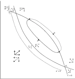
Output is normalized by capital stock to reflect the medium-run focus. The curves with = 0
and = 0 in Figure 1 represent the aggregate demand and supply curves facing the
representative firm. Their nonlinearity makes multiple equilibria or steady states with excess
capacity and positive mark- ups possible.
The specification of' the mark-up τ (see Equations A.13 and A.14) implies that τ is the profit
share and τ u the rental rate on capital.
6
With both investment and savings hyperbolic function of τ u and (sec the
appendix), the = 0 curve is convex to the origin.
We have the following restrictions on aggregate demand:
0,0 , 0, 0, , 0, = 0 = 0 (3)
[image:7.595.159.460.213.529.2]
Figure 1: The dynamic flow when mark-up varies inversely with u. Solid lines refer to the case of multiplier stability and dashed lines to the reverse. The curve on which u’ = 0 is the aggregate demand, andτ’ = 0 gives aggregate supply.
There is nothing in theory to rule out the case of 0, 0 or Keynesian multiplier
instability, where inducement to invest exceeds inducement to save, out of non-agricultural
income2. Even with this possibility, the output response need not be unstable and the firm
would maximize expected profits, provided some restrictions are placed on the price response
in Equation 2 (Goyal, 1993). These are:
2
Malinvaud (1983) sees an important link between multiplier instability, tamed by lags, and virtuous growth cycles. In the model developed here, a favourable growth scenario occurs with multiplier instability tamed by price setting behaviour
a
b
E1
u’ = 0
7
< 0, < 0, < 0and is large (4)
A brief rationale for Equation 4 follows.
1. If < 0 and is large, violent fluctuations in output are prevented even if 0.
Smooth adjustment paths, and a stable equilibrium E2 (Figure 1) exist. Only small
changes in the mark-up occur if is large.
2. If < 0, it is proved in Goyal (1993) that the firm maximizes expected profits over the
different possible adjustment paths. In such a case, downward sloping trajectories such
as b and a (Figure I) dominate. The variability of profit is less along such trajectories as
u and τ move in opposite directions. These more average profits would be preferred by
a risk-averse firm, compared to larger profit fluctuations along upward sloping
trajectories that dominate when 0. Also with < 0, recessionary downward
sloping trajectories of falling u and τ would be avoided.
3. < 0 ensures nonlinear adjustment to upper and lower bounds onτ.
4. For a monopolistically competitive firm, we have that the mark-up varies inversely
with the elasticity of demand. Even a competitive firm in disequilibrium faces a
demand elasticity of less than infinity. The mark-up is not ad hoc, but defines a virtual
pike (Neary and Roberts, 1980) that makes it optimal for the firm to produce at the
demand constrained output level. Higher investment and capital stock, in periods of
rising u, imply greater variability of output and a higher elasticity of demand. The
first-order conditions of short-run profit maximization of the firm then yield < 0 or
an inverse relationship between u andτ.
Figure I shows the aggregate demand, supply, and the dynamic flow when < 0. The dashed
lines indicate the case when Keynesian multiplier stability does not hold. As the partial
derivatives of the demand function change signs, a bifurcation occurs in the dynamic flow and
there is a switch from the low (a) to the high (b) growth trajectory. A growth cycle is made up
of ba and the trajectories joining them. Equilibrium E1 and E2 are saddle-stable, so that b and a
are unique paths (Goyal, 1993).
Why does a bifurcation take place? Rational expectations and other cross-equation restrictions
8
to exogenous demand or supply shocks. Endogenous difference-stationary growth cycles
occur.
It is hypothesized that, for the Indian economy, agricultural supply shocks, a decline in foreign
aid, and oil-price shocks from the mid-sixties led to a fall in public investment. Private
expected profitability fell. Rational expectations over altered expected adjustment paths led to
reduced private investment propensities (Goyal, 1993). The economy switched from trajectory
b approaching E2 to a approaching E1. In the mid-seventies the large inflow of remittances
from non-resident Indians led to a deliberate policy of budget deficits to run down foreign
reserves. Public investment increased, with domestic resource requirements met by a large
increase in domestic borrowing. That is the coefficient on private savings or τu in the public
investment function rose. The amplification effect outlined above worked in the reverse
direction and the economy switched once more to b.
3. Empirical Tests
Since the model is theoretical, highly aggregative and non-linear, it was decided to test it by
performing computer simulations using varying parameter value. The objectives were to test (i)
if the historical series could be replicated and estimates of likely parameter values obtained; (ii)
if the hypothesis of < 0 against 0held; (iii) if ≤ ; and (iv) if the economy
switched from b to a and back again.
Since the specification is unusual, (1) is indeed a test of its validity. The simultaneous equation
method of calibration (see Appendix) imposes more discipline than many single equation
estimates. The method is also broader than other calibration exercises since it involves the test
(ii) of competing theoretical hypotheses. The test (iii) is necessary since the endogenous
growth amplification effects would occur only if there were excess capacity. When = , the
dynamics change and the mark-up is the variable that now responds to excess demand
(Equation 2’) subject to a maximum, τmax. In the Indian economy for the period considered, it
was found that < . The capacity constrained case arises in some of the high growth counter
9
The equations were solved numerically using the classical fourth-order method of
Runge-Kutta. Simulations used Indian economic data3 for the period 1960/61 to 1984/85. The
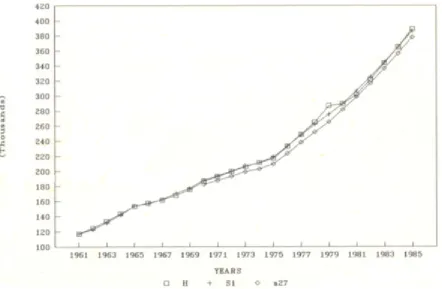
historical time series (H) for u and τ are quite closely reproduced by the simulated series SI.
Parameter values consistent with theoretical priors are obtained (see appendix). The trend of
the τ(H) series is captured. Short-run fluctuations are explained by lags in price-setting in other
simulations. The τ(H) series being derived from inadequate data is not very reliable, especially
after 1974/75. A number of alternative data sources are used as a check.
The parameter set A.d (see Appendix 4), with = − or < 0, generates series S I and
forms the basis for counterfactual simulations. The trajectories comprising S I approach E1 (for
the pre-1965/66 period), E2 (for 1965/66 to 1974/75), and E1 again post-1974/75. There is a
switch from b to a and back as hypothesized. The simulated trajectories in Figure 2 can be
compared to b a in Figure I.
3
10
Figure 2: Trajectories simulated for the Indian economy over the period 1960/61 to 1984/85 correspond to ab in Figure 1
Figure 3 (τ) also shows series S2 (generated by (A.d) with = or 0. They cannot
explain the perceptible rise in mark-ups that occurred in the late sixties. The simulations
reported in Figure 3 (τ) verify that only mark-up behavior with < 0 is capable of
reproducing the historical T series for the period 1965/66 to 1974/75. The τ(H) series after
1974/75 is not sufficiently reliable to discriminate between the simulations. Even so, the
simulations seem unable to falsify the weak hypothesis that when firms face declining demand
in the neighborhood of unstable multipliers, they will not decrease mark-ups for fear of
unstable price and output decreases.
Irrespective of whether 0, the mark-up behavior modelled was essential for stability in the
sense of prevention of large fluctuations in output. This is proved in simulations with the full
model where fixed prices lead to violent ahistorical short-run fluctuations in output.
The high value of w2 established implies a very gradual change in mark-up. Lower(higher)
values of w2 that generate a higher(lower) τ give rise to u which is lower(higher) than the
11
Figure 3: Simulations in (a) the output-capital ratio, u, (b) the mark-up, τ
4. Counterfactual High Growth Simulations
We examine the changes that would lead to higher growth in the model and the structure of
these high growth paths, first in the dynamic model and then in the extended AGEM. The latter
also allows us to look at aspects of agriculture-industry interactions, income distributional
changes, and inter-sectoral resource flows. Finally we draw together the implications for
12 4A. The structure of growth
Any simulation involving an increase in the inverse multiplierΩ would imply a switch to a
higher growth path. The change in Ω could be brought about by a rise in any of the investment
propensities or a fall in the saving propensity. Simulation S 11 in Table 1, reports the
percentage increase in some macroeconomic variables, resulting from a fall in f to 0.35 after
1964/65 (∼ 55 per cent rise in Ω). This simulation reconstructs the possible growth path if there
had been no dip in foreign inflows and public investment in the mid-sixties. Among the
conclusions from this and other simulations (see Goyal, 1989) are the following:
1. The percentage change in τ is less than one-third the percentage change in ym.
2. The influence of ym on Ipis greater than on IG, as a corollary Ipresponds more strongly
to a given change in IG through the effect of the latter on ym. There is complementarity
between Ipand IGin the long run, while high inflation and a resource squeeze can cause
reverse crowding out of public sector investment.
3. Change in Ω is much stronger than that of equivalent changes in e. To generate an
equivalent growth path would require a 6 to 16 times higher initial investment in the
latter case. A ‘big push’ in investment is not essential. It is adequate for high growth
that investment should rise as a reasonably high percentage of output.
4. The relatively small changes in τ indicate that cost-push factors are the major cause of
inflation.
5. Reversible shocks have persistent long run effects or difference stationary growth
cycles occur.
The dynamic model was used to determine non-agricultural output and prices in the AGEM
developed by Narayana et.al (1991) for agricultural policy analysis. In the AGEM,
non-agricultural output and prices are given by historical data for the period 1969/70 to
1984/85, over which it is calibrated. After that non-agricultural output is determined by
capacity which is a function of past investment while prices remain fixed. The dynamic model
allows output to be the minimum of demand or capacity, and also endogenizes non-agricultural
prices. The latter are obtained by applying the mark-up to historically given labor-output ratios
13
Agricultural price and output is now endogenized through empirically estimated demand and
supply curves. Supply in agriculture is fixed in one period and changes in the next. Income
distribution is also endogenized, so that relative prices change as both the level and the
distribution of income changes in the high growth simulations.
Since a demand system is not estimated for non-agricultural output, relative price effects on
non-agricultural consumption demand are not captured. The real value of endogenous
household saving and residual government dissaving depends on non-agricultural price.
Effects of agricultural output and terms of trade on investment and saving are still kept in the
exogenous part, e. As they enter with opposite signs they cancel out. The long-run agricultural
supply response is higher than the short-run, as the share of investment in agriculture responds
to changes in terms of trade. The price elasticity is only 0.25. The share is largely determined
by a time trend that captures the historical share of agriculture in investment that has been
around 18-20 percent in the eighties.
A key to the major simulations presented in Table 1 follows: S 11- f reduced to 0.35 from
1964/65, a17 - i1 increased 5 percent from 1974/75, a27 - base run with (A.d), a28 - f = 0.35
with base a27, and al9 -f = 0.35, capital-output ratio, k = 5/(1.01)t. S prefixes simulations with
only the dynamic model, a, those with the full model. All simulations are based on the
parameter set (A.d), with the changes in each indicated below. The initial year is 1960/61 for
simulations with the dynamic model and 1969170 for the extended model.
Figures 3 and 4 report the results of one simulation, a27, with 1969-70 as the initial period.
Despite the different initial period, which could make a difference as the model is nonlinear,
the resulting series follow the trend of both S1 and the historical series. Moreover, simulation
a28 with f = 0.35 from 1969-70, gives results comparable to S11 (in Table 1). Other
simulations (not reported for reasons of space) reinforce these results. Simulation results are
firmer if they hold for a range of parameter values and doubly so if they hold in a different
1
4
Table 1: Percentage change over base run
Experiment Percentage
change
over base
run in year
ym u τ Ip Ig Inom s(τymPm) Pm Pa Pa/Pm TSAVE(nom) ya GCSV(nom)
(1) (2) (3) (4) (5) (6) (7) (8) (9) (10) (11) (12) (13) (14) (15)
S 11 1970-71 8.7 7.2 -2.7 3.0 12.1 6.6* 2.9* -2.1 - - - - -
1984-85 32.1 20.2 -8.5 16.2 24.5 20.2* 12.4* -6.4 - - - - -
a 17 1984-85 8.3 7.2 -2.8 60 1.4 1.4 2.0* -2.3 4.9 5.9 9.9 - -32.3
a 28 1984-85 37.0 20.0 -8.7 17.9 25.6 13.1 13.0 -6.9 37.8 49.3 60.9 1.1 -193.3
1998-99 43.6 18.3 16.2 54.9 68.0 83.1 79.4 14.1 -3.9 -16.7 49.3 3.1 0.0
a 19 1984-85 42.6 34.8 -14.4 11.4 20.0 3.0 8.9* -10.8 36.8 37.3 58.5 -9.4 -210.9
1991-92 67.8 52.0 -26.4 14.5 25.8 -1.4 11.8* -17.5 47.5 47.5 71.1 -8.1 -184.6
1994-95 71.1 52.2 -26.4 18.9 31.1 2.8 15.7* -16.1 120.0 121.0 74.5 -15.8 -169.2
15
Figure 4: Simulations in output, ym
4B. Agriculture and resource flows
The structure of the AGEM allows a number of new issues to be considered: (1) the effect of
relative prices on demand and growth; (2) the short- and long-run agricultural supply response;
(3) the interaction between changes in income distribution and growth; and (4) the investment
and savings flows between agriculture and non-agriculture.
In Table 1 column 11, agricultural prices increase with non-agricultural output and respond
steeply to a large rise in the latter, but the supply response (column 14) is low. It is higher in the
long run, but can even be negative for a steep rise in agricultural prices. In a28, full capacity
output, (with a capital-output ratio of 5) is reached in 1983-84 after which non-agricultural
output grows more slowly. Agricultural terms of trade, after rising steeply, fall below the base
run by 1990-91. Agricultural output, which is often below the base run is only 3 percent higher
by 1998-99 as a result of increased investment. In a19, again with f = 0.35, allowance is made
for rising productivity with the capital-output ratio falling to reach 3.8 by 1992/93, when the
capacity constraint is binding. Even so, demand once more falls below capacity by 1994/95,
16
In a 19, the rates of growth of output (columns 3 and 4), are much higher than in a 17. In the
former, supply-side productivity growth, due to new technology or increasing returns to scale
allows growth in Full capacity is not reached until 1992/93, so that accelerated demand led
growth is feasible until then. Demand cycles arc embedded in supply cycles. The higher
productivity of capital and falling mark-ups mean that the rise in investment is lower in a 19,
compared to a 28 [columns (6) and (7)]. At the same time, in the former there is a steep rise in
the agricultural terms of trade, but a fall in agricultural output. Substitution in consumption,
and short- and long-term supply response to relative price changes is inadequate to adjust
agricultural demand to supply, given the slow growth in investment. Narayana et. al. (1991)
show that raising investment in agriculture and targeting it towards improving the irrigation
potential leads to the largest increase in agricultural output.
In the dual economy literature it is established that agriculture can serve as a source of demand
for industry if the level of income in agriculture is high and evenly distributed and the price
elasticity of food demand is not too low. Neither of these conditions holds for India. In the
absence of a rise in agricultural supply, the wage-goods constraint can squeeze non-agricultural
demand and profits.
Most dual economy models neglect investment in agriculture. As the majority of investment
goods are produced in non-agriculture, a rise in agricultural investment is a source of demand
for industry and at the same time, eases the wage goods constraint. A number of studies show
that private and public investment in agriculture are complimentary. In India the share of
agriculture in both has been declining since the late seventies. That the very large rise in
agricultural prices is unable to choke off demand is indirect evidence of the low price elasticity
of agricultural demand in India. Increase in public expenditure, apart from investment, cannot
be very effective in inducing a rise in demand for industry given the leakage of expenditure to
items of food.
The dynamic model showed a gap between investment and savings in each year, which was
close to the historical gap and was probably caused by data and deflation problems (Goyal,
1989). The AGEM imposes balance in physical and financial flows for each of 10 rural, urban
income groups, ten commodity sectors, the government, and the aggregate investment savings
17
that none of the balance conditions arc violated in the higher growth dynamic simulations
unless there is extreme disproportion between the sectoral rates of growth.
It is also notable that nominal total household savings (TSAVE) exceeds investment in most
periods so that nominal government savings (GCSV) arc negative. The latter implies that
savings are effectively determined by investment. It is even more interesting that in the higher
growth scenarios, TSAVE grows faster than investment so that GCSV becomes more negative
(see a19, Table 1). In a28 GCSV finally approaches its base run values as growth slows with
the capacity constraint holding. The increase in TSAVE exceeds that in savings out of profit
income, S. This means that the dynamic growing non-agricultural sector can invest in excess of
its savings and attract savings from other sectors. Growth can finance itself.
Are the estimates of TSAVE realistic? Narayana et al. (1991) estimate a jointly log-normal
distribution of consumption and income that reconciles NCAER (1980) data on cross-sectional
income distribution for 1975/76 and C.S.O. time series. This is used to determine the
proportion of population, consumption, and savings in different income groups separately for
rural, urban and rural non-agricultural population. Table 2 shows how the population and per
capita saving vary in different simulations. An important source of the rise in TSAVE is the
increase in population in the upper income groups with growth. This aspect is not adequately
captured in the normal aggregative macroeconomic savings function. If the parameters of the
distribution function change so that the lower income groups benefit more from growth,
through increased employment generation the increase in TSAVE would be lower. If there is a
larger shift of population to the urban sector, TSAVE would increase. The large numbers that
remain in the lower income groups of the rural population, even with high growth indicates that
high non-agricultural growth is not sufficient to remove rural poverty. Special measures are
required for the agricultural sector. The rise in agricultural prices has an adverse effect on the
lower income groups, and in a27 the gini coefficient is first higher and then lower than in the
base run.
18
Macroclosure issues in this paper can be defined in two different ways: (i) the investment
savings balance and its interaction with government finances; and (ii) the rigidity of mark-ups
and large quantity variations derived from optimization decisions over disequilibrium
adjustment paths. The effect of disequilibrium on the endogenous variables is simply captured
[image:19.595.70.532.222.602.2]without explicitly modeling money and credit markets.
Table 2: Population (in m) and Per Capita Savings (S/c) (in current prices), by Income Groups
Income Classes Experiment Year ≤≤≤≤ Rs. 216 > Rs. 216
≤ ≤ ≤
≤ Rs. 336
> Rs. 336 ≤
≤≤
≤ Rs. 516
> Rs. 516 ≤
≤ ≤
≤ Rs. 900
> Rs. 900
Rural 1984-85
a27 Population 200.88 103.04 102.95 100.27 49.79
S/c -16.84 120.60 402.75 1180.86 4177.70
1998-99
Population 199.37 108.88 124.89 156.98 118.03
S/c — — — — 3834.30
Urban 1984-85
a27 Population 8.45 23.34 44.24 61.36 42.72
S/c -16.46 14.06 225.27 839.65 3679.24
1998-99
Population 3.86 18.02 54.10 117.44 124.13
S/c — — — — 3758.40
Rural 1984-85
a28 Population 200.22 100.81 97.16 97.51 61.23
S/c -16.84 121.05 410.30 1246.60 5728.90
1998-99
Population 200.10 108.42 118.20 132.31 149.11
S/c -30.30 44.20 224.32 889.10 4734.80
Urban 1984-85
a28 Population 3.74 14.56 35.71 64.13 61.98
S/c -61.99 13.02 229.23 874.91 4244.30
1998-99
Population 1.31 8.33 33.65 101.94 172.32
S/c -68.51 -18.98 149.40 725.43 4667.20
On the high growth paths, savings exceeded investment and the public sector was a net
dissaver. In the Indian economy the latter has indeed been the case. With borrowing supporting
even current expenditure and low returns from public sector investment, public debt was
reaching unsustainable levels. The stabilization imposed in the nineties seeks to bring down the
fiscal deficit. Unfortunately the latter is being attempted by cut down of public investment and
privatization, without controlling the revenue deficit. The privatization attempts have been
19
investment. If high public sector investment could, according to the counterfactuals analyzed
in this paper, maintain high growth, resources to finance it could be allocated to the public
sector by privatization. While the stock of public sector capital would be unchanged, its share
could fall as private investment also rose. This happened in Taiwan. The sale of shares in select
enterprises, together with other market structure reform would help to increase the efficiency
of public enterprises. There is some evidence that in periods of low growth, resources flow into
speculative activities (Goyal, 1992). With greater openness, foreign inflows would also be
more easily attracted by high growth. In the current agriculture-industry model, flows between
the two must balance. We have seen how investment in agriculture lead by public sector
investment would be balanced by agricultural savings flowing into the non-agricultural sector
on a high growth path. Simulation a19 suggests that the current policy initiative of giving
farmers higher prices may not succeed if not supported by a rise in investment.
Since the non-agricultural sector is not disaggregated, the mark- up decision of the
representative firm reflects macroeconomic forces that impinge on its expected demand. Given
the structure of the model, the latter, in turn, is directly determined by investment and savings
dynamics. Focusing on the latter makes possible a medium-run perspective, rather than that of
short-run macro-monetary fluctuations. There is some empirical evidence about the better
performance or macro- relative to micro-variables in firms’ decisions4. The above analysis may
be valid even leaving the representative firm framework, with a more disaggregated
non-agricultural sector. The mark-up in each sector would be determined by its market
structure, and dynamic macroeconomic considerations.
In AGE models, it becomes difficult to explain or calibrate the model to observed country
high-growth experiences in the Walrasian framework. Recent work has tended to impose
arbitrary supply-side increasing returns to scale or technology shocks. The model in this paper
uses endogenous demand-side intensifications of growth, caused by either demand or supply
shocks.
4
20
In the dynamic model, the mark-up is endogenized and found to be relatively rigid and
countercyclical. The price level is normalized at one for the base period. Endogenizing money
wages and linking them to agricultural prices could explain the price level.
The combined insights of the dynamic and AGE models lead to the following policy
conclusions:
1. It is feasible to shift to a higher growth path provided less costly means are devised to
improve the allocation of savings to the public sector, and sustain investment increases.
As both the quantity and allocation of savings is responsive to high growth and
profitability, sale of public sector enterprises would be feasible on a high growth path
and could be used to maintain high public investment.
2. Allocation of investment for irrigation and employment in agriculture should be
increased to control rise in prices and their adverse income distributional, growth, and
political consequences.
3. A new approach to policy in line with the mechanism design literature is desirable.
Policy should seek to identify feasible variation in parameters that, by changingΩ,
would change the dynamics of the system. Growth could intensify and/or a favorable
bifurcation could occur in the growth path.
5. Conclusion
In this paper by using a simple technique to model disequilibrium without modeling money
markets explicitly we (i) suggest a possible solution to the closure debate, (ii) obtain relatively
rigid counter cyclical mark-ups in a theoretically consistent way, (iii) show that, given the
latter, investment savings dynamics can explain endogenous growth amplifications, and (iv)
use the model to explain growth paths for the non-agricultural sector of the Indian economy.
Counterfactual simulations (i) with the dynamic model (ii), putting the latter in an agricultural
policy AGEM show:
1. Public sector investment 'crowds in' private sector investment, and is itself crowded out
in periods of resource constraint. Both are complementary in agriculture.
2. In Indian agriculture, at least historically, supply response to the terms of trade has been
21
3. On counterfactual high-growth paths without increase in investment in agriculture there
is no alleviation of rural poverty and a steep rise in agricultural terms of trade with
adverse effects on growth.
4. On the high-growth simulations household savings exceed investment.
5. Savings required for successful privatization would flow to the public sector if the
proceeds were used to maintain high public-sector investment with a large allocation to
agriculture. The latter would be a prerequisite for high growth until structural
adjustment successfully changes the dynamics of the system.
APPENDIX
1. The One Period Model
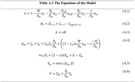
The endogenous price and quantity variables in a given period are determined by Equations
A.1 to A.14 in Table A.1. The symbols are defined in Sections 1A-1C. Equation A.1 gives the
short-run non-agricultural mark-up n as the excess of non-agricultural price over direct,
indirect labor input coefficient, and profits are n ym. The equation shows that price in a given
period may be fixed as a function of long-run mark-upτ. These equations are the first-order
conditions of profit maximization by the representative firm. The long-run mark-up τ will
differ from n only if price is a lagged function of costs, was taken to be the case in some
simulations.
Equation A.2 builds up the capital stock in non-agriculture as sum of last period capital stock
and investment in non-agriculture, subtracting the part of investment going to agriculture.
Capacity output is obtained from the capital stock, given an output-capital ratio.
The rest of the equations determine output and its components. In A4, aggregate demand for
non-agricultural output is built up as a of all the standard categories minus net imports of
industrial products, Fm. Investment is broken up into that originating in the private and that in
the public sector. Consumption is broken up into consumption of non-agricultural output out of
agricultural income, wage income foreign inflows, and profit income. It is assumed that
workers consume all their income and have a fixed minimum consumption of agricultural
22
Non-agricultural output is the minimum of demand or capacity (A.5) and along with
agricultural output (exogenous) adds up to total output. Public sector investment (A.7) is
derived from the government budget constraint. Given restrictions on inflationary deficit
finance and dependence on institutional and other market borrowing, it is an increasing
function of the different categories of savings, and a decreasing function of rise in agricultural
prices. Private sector investment (A.8) is obtained from the representative firm's maximization
of expected net cash flow subject to a probability of making sales. It is an increasing function of
profits and a decreasing function of excess capacity. This is equivalent to the ‘q’ theory of
investment with excess capacity adding an opportunity cost element to adjustment costs5. An
implication of this specification is that to ! . Savings (A.10-A.12) is broken up into
domestic and foreign savings, and savings out of non-agricultural profit income, and
agricultural income. Consumption/savings behaviour is derived from consumer utility
maximization under employment and liquidity constraints. Quantities are measured in money
(Rupees) with Pmas the numeraire, so that all variables expect Ware in units of non-agricultural
[image:23.595.64.532.415.699.2]output.
Table A.1 The Equations of the Model
" = −$ %# &−$ % −$ $$ %&' &'−$ %$( (−$ %) * (A.1)
+! = +!,&+ !,&− ./ !,& (A.2)
= 0+ (A.3)
1 = 2+ ( + 3 4 $ + 5 − 6 %$ $# − 6−$$ 7
+6898+ − : "4 + ; − 9
(A.4)
4 = <=". 1 , (A.5)
4 = 4 +$ 4$ (A.6)
5
23
( = (*+ & − :" +$ : 4$
+ 8$ + 9& & 0, 8 < 0
(A.7)
2 = 2*+ ? <=". 1 , − + =&" + =898 ?, =&, =8 0 (A.8)
= (+ 2 (A.9)
@ = :" + : $ +$ ( (A.10)
A = 9&+ :898 (A.11)
= @+ A (A.12)
B = −$ %# = " (A.13)
$ = %# −C (A.14)
= D + =&+ &: − − : + ? (A.15)
= & − 8 8+ E & 0, 8 0, E ≥ 0 (A.16)
D = D( + D2− DG (A.17)
D( = (*+ 8$ + 9&+ &: D − /+′ (A.18)
D2 = 2*+ =898− JK /+ (A.19)
DG = (+ A+ : D − /+ (A.20)
D = $ / #%&+ $ % + $&'%&'+ $(%( + )%L (A.21)
1A. Endogenous variables (equal to number of equations)
n = fixed price mark-up for non-agriculture
K = capital stock in non-agriculture
= capacity output of non-agriculture
dm = demand for non-agriculture
ym = output of non-agriculture
y = total output
24 Ip = investment by the private sector
I = total investment
SD = domestic savings
SF = savings out of foreign inflows
S = total savings
= total profits in non-agriculture
Pm = price level of the non-agriculture sector
u = C , = ++ C
τ = mark-up in non-agriculture
eG, ep, es = constituents of IG, Ip, S respectively taken as exogenous in the dynamic model
e = the exogenous part of aggregate I minus S
eτ = ratio of Pa to all per unit input costs
1B. Exogenous Variables
W = money wage rate
Pa = price level of the agricultural sector
PIM = price level of intermediate imports
PG = price of intermediate inputs produced in the public sector
r = nominal rate of interest
v = full-capacity output-capital ratio in non-agriculture
Iagr = investment in agriculture
ye = output of the agricultural sector
G = government consumption expenditure
T = government taxes
F = foreign inflows, F = F1 + F2, in units of non-agricultural product
Fm = imports in excess of non-agricultural exports
F1 = foreign inflows to the public sector
F2= foreign inflows to the private sector
P*a = dPa/dt a superscript dash always indicates a time derivative
SG = public sector savings
1C. Parameters
25 aa = agricultural raw materials per unit of ym
aIM = intermediate imports per unit of ym
aK = intermediate inputs (produced in the public sector) per unit of ym
aK = working capital per unit of ym
cm = propensity to consume non-agricultural goods out of agriculture income
ca = propensity to consume agricultural output out of wage income in non-agriculture
a = direct and indirect labor requirements per unit of ym
6M = fixed consumption of agricultural products by workers in non-agriculture c2 = propensity to consume out of F2
s = propensity to save out of profit income in non-agriculture
g1= public sector propensity to invest out of private sector savings
g2= the effect on I of the rate of growth of agricultural prices
sa = propensity to save out of agricultural incomes
f = a dummy variable effecting the public sector propensity to invest out of savings in the
manufacturing sector
j = a parameter capturing the effect of aggregate demand in relation to capacity on Ip
i1 = private sector propensity to invest out of profit income
i2 = private sector propensity to invest out of F2
w1, w2, w3 = parameters of theτ ’
function
2. The Dynamic Model
Equation A.IS models the adjustment of non-agricultural output equate savings to investment,
all normalized by capital stock. The exogenous parts of investment and savings, which are
functions of agricultural income and price, intermediate input prices, and foreign inflow, are
gathered together in the e terms (A.17-A.21), and u' becomes a nonlinear function of u and τ.
As a simplifying assumption, terms of trade effects on agricultural savings are treated as
exogenous. The dynamics are dominated by the termΩ = =&+ &: 1 − − : + ?, which
is the negative of the inverse of the Keynesian short-run multiplier.
3. Calibration
Historical time series for the endogenous variables, the exogenous series of the e’s, W, a, Iagr
and initial values of u τ, K were derived from C.S.O, R.B.I., B.S.l.E. and other sources of data,
26
the investment, savings and τ' equation parameters that reproduced the historical series were
isolated. The e series were calculated by subtracting the endogenous components of investment
and savings from the respective historical series. The calibrated model was then used as a base
for counterfactual simulations. The same exogenous series were used in simulations with the
AGEM, but the initial period was 1969/70.
4. The Calibrated Parameter Set
Inverse multiplier (Ω) values that generate close approximations to the historical data series are
pre-1965/66 = .0194, 1965/66 to 1974/75= -0.0235, post-1974/75 = 0.00546, if τ = .4.
Parameter values commensurate with these values of omega and the historical series on saving
and investment are:
1. For 1960/61 to 1974/75:, i1 = 0.258, j = 0.002, s = 0.429, g1 = 0.5, w2 =0.9, with f = 0 for
1960/61 to 1964/65 and f = 0.5 thereafter:
2. For 1975/76 to 1984/85:
i1 = 0.32, j = 0.002, s = 0.479, g1 = 0.7, w = 0.9, with f = 0.5 throughout. (A.d)
Sensitivity analysis confirmed these values
References
Dewatripont, M., and Michel, G. (1987) On Closure Rules, Homogeneity and Dynamics in Applied General Equilibrium Models. Journal of Development Economics 26: 65-76.
Goyal, A. (1989) The Short-Run Behaviour of the Indian Economy and its Implications for Long-run Growth. Unpublished Ph.D. Dissertation. Bombay University.
Goyal, A. (1992) Demand, Supply and Savings Constraint in the Indian Economy. Economic and Political Weekly 27: 893-899.
Goyal, A. (1993) Stability Expectations and Bifurcations: A Characterization of
Disequilibrium Growth Paths. Indira Gandhi Institute of Development Research discussion paper, 90.
Grunfeld, Y., and Griliches, Z. (1960) Is Aggregation Necessarily Bad? Review of Economics and Statistics 42: 1-13.
Malinvaud, E. (1980) Profitability and Unemployment, Cambridge: Cambridge University Press.
Malinvaud, E. (1983) Notes on Growth Theory with Imperfectly Flexible Prices. In Modern Macroeconomic Theory (Fitoussi, Ed.). Oxford: Basil Blackwell.
27 Press,
Narayana, N.S.S., Parikh, K.S., and Srinivasan, T.N. (1991) Agriculture, Growth and Re- distribution of Income: Policy Analysis with a General Equilibrium Model of India. Allied Amsterdam: Publishers, New Delhi/North Holland.
Neary, R., and Roberts, K. W.S. (1980) The Theory of Household Behaviour Under Rationing. European Economic Review 13: 25-42.