Quintic B-Spline Collocation Method for Tenth Order
Boundary Value Problems
K.N.S.Kasi Viswanadham
Department of Mathematics National Institute of Technology
Warangal – 506004 (INDIA)
Y.Showri Raju
Department of Mathematics National Institute of Technology
Warangal – 506004 (INDIA)
ABSTRACT
A finite element method involving collocation method with quintic B-splines as basis functions has been developed to solve tenth order boundary value problems. The fifth order, sixth order, seventh order, eighth order, ninth order and tenth order derivatives for the dependent variable are approximated by the central differences of fourth order derivatives. The basis functions are redefined into a new set of basis functions which in number match with the number of selected collocated points in the space variable domain. The proposed method is tested on several linear and non-linear boundary value problems. The solution of a non-linear boundary value problem has been obtained as the limit of a sequence of solutions of linear boundary value problems generated by quasilinearization technique. Numerical results obtained by the present method are in good agreement with the exact solutions available in the literature.
Keywords
Collocation Method; Quintic B-spline; Basis Function; Tenth Order Boundary Value Problem; Absolute Error.
1. INTRODUCTION
The higher order boundary value problems are known to arise in hydrodynamic, hydro magnetic stability and applied sciences. It is well known that when a layer of fluid is heated from below and is subject to the action of rotation, instability may set in as ordinary convection which may be modelled by a tenth-order boundary value problem. In addition, ultrasonically assisted development of resists feature on semiconductor substrate is a popular development technique, but is difficult to understand. During this development process the developer i.e. 1:3 Methyl isobutyl Ketene and Isopropyl alcohol is heated because of ultrasonic agitation. During heating an infinite horizontal layer of fluid and then subjecting to the action of rotation, instability sets in. When this instability sets as an ordinary convection and a uniform magnetic field is also applied across the fluid in the same direction as gravity, then the problem is modelled by a tenth-order boundary value problem [1].
In this paper, we developed a collocation method with quintic B-splines as basis functions for getting the numerical solution of a general linear tenth order boundary value problem
a0(x)y(10)(x) + a1(x)y(9)(x) + a2(x)y(8)(x) + a3(x)y(7)(x) + a4(x)y(6)(x) + a5(x)y(5)(x) + a6(x)y(4)(x) + a7(x)yʹʹʹ(x) + a8(x)yʹʹ(x) + a9(x)yʹ(x) + a10(x)y(x) = b(x), c<x<d (1) subject to the boundary conditions
y(c) = A0, y(d) = B0, yʹ(c) = A1, yʹ(d) = B1,
yʹʹ(c) = A2, yʹʹ(d) = B2, (2) yʹʹʹ(c) = A3, yʹʹʹ(d) = B3,
y(4)(c) = A4, y (4)
(d) = B4
where A0, B0, A1, B1, A2, B2, A3, B3, A4, B4 are finite real constants and a0(x), a1(x), a2(x), a3(x), a4(x), a5(x), a6(x), a7(x), a8(x), a9(x), a10(x) and b(x) are all continuous functions defined on the interval [c, d].
Volume 51– No.15, August 2012 boundary value problems. Solution of linear and nonlinear
boundary value problems of tenth and twelfth-order was implemented by Wazwaz [13] using adomian decomposition method. Numerical methods for special nonlinear boundary value problems of order 2m are developed by Djidjeli et. al.[14].
The above studies are concerned to solve tenth order boundary value problems by using tenth or eleventh order B-splines. In this paper, quintic B-splines as basis functions have been used to solve the boundary value problems of the type (1)-(2).
In section 2 of this paper, the justification for using the collocation method has been mentioned. In section 3, the definition of quintic B-splines has been described. In section 4, description of the collocation method with quintic B-splines as basis functions has been presented and in section 5, solution procedure to find the nodal parameters is presented. In section 6, numerical examples of both linear and non-linear boundary value problems are presented. The solution of a nonlinear boundary value problem has been obtained as the limit of a sequence of solutions of linear boundary value problems generated by quasilinearization technique [15]. Finally, the last section is dealt with conclusions of the paper.
2. JUSTIFICATION FOR USING
COLLOCATION METHOD
In finite element method (FEM) the approximate solution can be written as a linear combination of basis functions which constitute a basis for the approximation space under consideration. FEM involves variational methods such as Ritz’s approach, Galerkin’s approach, least squares method and collocation method etc. The collocation method seeks an approximate solution by requiring the residual of the differential equation to be identically zero at N selected points in the given space variable domain where N is the number of basis functions in the basis [16]. That means, to get an accurate solution by the collocation method, one needs a set of basis functions which in number match with the number of collocation points selected in the given space variable domain. Further, the collocation method is the easiest to implement among the variational methods of FEM. When a differential equation is approximated by mth order B-splines, it yields (m+1)th order accurate results [17]. Hence this motivated us to solve a tenth order boundary value problem of type (1)-(2) by collocation method with quintic B-splines as basis functions.
3. DEFINITION OF QUINTIC B-SPLINES
The cubic B-splines are defined in [18, 19]. In a similar analogue, the existence of the quintic spline interpolate s(x) to a function in a closed interval [c, d] for spaced knots (need not be evenly spaced) c = x0 < x1 < x2 < … < xn-1 < xn = d is established by constructing it. The construction of s(x) is done with the help of the quintic B-splines. Introduce ten additional knots x-5, x-4, x-3, x-2, x-1, xn+1, xn+2, xn+3, xn+4 and xn+5 such that
x-5 < x-4 < x-3 < x-2 < x-1 < x0
and xn < xn+1 < xn+2 < xn+3 < xn+4 < xn+5.
Now the quintic B-splines Bi(x)'s are defined by
otherwise 0
] x , [x x if ) (
) (
B i-3 i3
3 3
' 5 i
i i r r
r
x x x
x
where
x
x
if
0
x
x
if
)
x
x
(
)
x
x
(
r r 5 r 5 r
and
3 3
r) x -x ( ) x (
i i r
.
It can be shown that the set {B-2(x), B-1(x), B0(x), …, Bn(x), Bn+1(x), Bn+2(x)} forms a basis for the space
S
5(
)
of fifth degree polynomial splines. The quintic B-splines are the unique non-zero splines of smallest compact support with knots atx-5 < x-4 < x-3 < x-2 < x-1 < x0 < … < xn < xn+1 < xn+2 < xn+3 < xn+4 < xn+5.
4. DESCRIPTION OF THE METHOD
To solve the boundary value problem (1)-(2) by the collocation method with quintic B- splines as basis functions, we define the approximation for y(x) as
) x ( B )
x ( y
2
2 j
n
j j
(3)where αjʹs are nodal parameters to be determined. In the present method, the internal mesh points x3, x4, …, xn-3 are selected as the collocation points. In collocation method, the number of basis functions in the approximation should match with the number of collocation points[16]. Here the number of basis functions in the approximation (3) is n+5, where as the number of selected collocation points is n-5. So, there is a need to redefine the basis functions into a new set of basis functions which in number match with the number of selected collocation points. The procedure for redefining the basis functions is as follows:
Using the quintic B-splines described in section 3 and the Dirichlet boundary conditions of (2), we get the approximate solution at the boundary points as
0 0 2
2 j
0) B (x )
y(x )
(c A
y
j
j
(4)0 n 2
2 j
n) B(x )
y(x )
(d B
y
n
n j
j
. (5)Eliminating α-2 and αn+2 from the equations (3), (4) and (5), we get the approximation for y(x) as
)
x
(
P
)
x
(
w
y(x)
j1
1
1
nj j
where
)
x
(
B
)
x
(
B
B
)
x
(
B
)
x
(
B
A
)
x
(
w
n 2n 2 n
0 2
-0 2
-0
1
. 1. n n, 1, -n 2, -n j , ) x ( B ) x ( B ) x ( B ) x ( B 3 -n 3,4,..., j , ) x ( B 1,0,1,2 -j , ) x ( B ) x ( B ) x ( B ) x ( B ) x ( P 2 n n 2 n n j j j 2 -0 2 -0 j j j for for for
Using the Neumann boundary conditions of (2) to the approximation y(x) in (6), we get
yʹ(c) = yʹ(x0) = w1ʹ(x0) + α-1P-1ʹ(x0) + α0P0ʹ(x0) + α1P1ʹ(x0) + α2P2ʹ(x0) = A1 (7) yʹ(d) = yʹ(xn) = w1ʹ(xn)+αn-2Pn-2ʹ(xn)+ αn-1Pn-1ʹ(xn)+αnPnʹ(xn) + αn+1Pn+1ʹ(xn)= B1. (8) Now, eliminating α-1 and αn+1 from the equations (6), (7) and (8), we get the approximation for y(x) as
)
x
(
Q
)
x
(
w
y(x)
j 0 2
n j j
(9)where ) x ( P ) x ( P ) x ( w B ) x ( P ) x ( P ) x ( w A ) x ( w (x)
w n1
n ' 1 n n ' 1 1 1 -0 ' 1 -0 ' 1 1 1 2 and . n 1, -n 2, -n j , ) x ( P ) x ( P ) x ( P ) x ( P 3 -n 3,4,..., j , ) x ( P 0,1,2 j ), x ( P ) x ( P ) x ( P ) x ( P ) x ( 1 n n ' 1 n n ' j j j 1 -0 ' 1 -0 ' j j for for for Qj
Using the boundary conditions yʹʹ(c) = A2 and yʹʹ(d) = B2 of (2) to the approximate solution y(x) in (9), we get
yʹʹ(c) = yʹʹ(x0) = w2ʹʹ(x0) +α0Q0ʹʹ(x0) +α1Q1ʹʹ(x0) +α2Q2ʹʹ(x0) = A2 (10) yʹʹ(d) = yʹʹ(xn) = w2ʹʹ(xn)+αn-2Qn-2ʹʹ(xn) +αn-1Qn-1ʹʹ(xn)
+αnQnʹʹ(xn) = B2. (11) Now, eliminating α0 and αn from the equations (9), (10) and (11), we get the approximation for y(x) as
)
x
(
R
)
x
(
w
y(x)
j 1 1 3
n j j
(12)where ) x ( Q ) x ( Q ) x ( w B ) x ( Q ) x ( Q ) x ( w A ) x ( w (x) w n n '' n n '' 2 2 0 0 '' 0 0 '' 2 2 2 3 and 1. -n 2, -n j , ) x ( Q ) x ( Q ) x ( Q ) x ( Q 3 -n 3,4,..., j ), x ( Q 1,2 j ), x ( Q ) x ( Q ) x ( Q ) x ( Q ) ( n n '' n n '' j j j 0 0 '' 0 0 '' j j for for for x Rj
Now, using the boundary conditions yʹʹʹ(c) = A3 and yʹʹʹ(d) = B3 of (2) to the approximate solution y(x) in (12), we get
yʹʹʹ(c) = yʹʹʹ(x0) =w3ʹʹʹ(x0) + α1R1ʹʹʹ(x0) + α2R2ʹʹʹ (x0)
= A3 (13) yʹʹʹ(d) = yʹʹʹ(xn) =w3ʹʹʹ(xn) + αn-2Rn-2ʹʹʹ(xn) + αn-1Rn-1ʹʹʹ(xn) = B3. (14) Now, eliminating α1 and αn-1 from the equations (12), (13) and (14), we get the approximation for y(x) as
)
x
(
S
)
x
(
w
y(x)
j 2 2 4
n j j
(15)where
)
x
(
R
)
x
(
R
)
x
(
w
B
)
x
(
R
)
x
(
R
)
x
(
w
A
)
x
(
w
(x)
w
1 -n n '' ' 1 -n n '' ' 3 3 1 0 '' ' 1 0 '' ' 3 3 3 4
and
2.
-n
j
,
)
x
(
R
)
x
(
R
)
x
(
R
)
x
(
R
3
-n
3,4,...,
j
),
x
(
R
2
j
),
x
(
R
)
x
(
R
)
x
(
R
)
x
(
R
)
(
1 -n n '' ' 1 -n n '' ' j j j 1 0 '' ' 1 0 '' ' j jfor
for
for
x
S
jNow, using the boundary conditions y(4)(c) = A4 and y(4)(d) = B4 of (2) to the approximate solution y(x) in (15), we get y(4)(c) = y(4)(x0)= w4
(4)
(x0)+α2S2 (4)
(x0)=A4 (16) y(4)(d) = y(4)(xn)= w4
(4)
(xn)+αn-2 Sn-2 (4)
(xn)=B4. (17) Now, eliminating α2 and αn-2 from the equations (15), (16) and
(17), we get the approximation for y(x) as
)
x
(
B
~
w(x)
y(x)
j 3 3 j j
n
(18)where
)
x
(
S
)
x
(
S
)
x
(
w
B
)
x
(
S
)
x
(
S
)
x
(
w
A
)
x
(
w
w(x)
2 -n n (4) 2 -n n (4) 4 4 2 0 (4) 2 0 (4) 4 4 4
and)
(
)
x
(
B
~
j
S
jx
, for j=3,4,…,n-3.Now the new basis functions for the approximation y(x) are
3 ,..., 4 , 3 ), ( ~ n j x
Bj and they are in number match with
the number of selected collocated points. Since the approximation for y(x) in (18) is a quintic approximation, let us approximate y(5), y(6), y(7), y(8), y(9) and y(10) at the selected collocation points with central differences as
(4)
3Volume 51– No.15, August 2012
5) 4 ( 3 ) 4 ( 2 ) 4 ( 1 ) 4 ( 1 ) 4 ( 2 ) 4 ( 3 ) 9 ( 4 ) 4 ( 2 ) 4 ( 1 ) 4 ( ) 4 ( 1 ) 4 ( 2 ) 8 (
2
/
)
4
5
5
4
(
/
)
4
6
4
(
h
y
y
y
y
y
y
y
h
y
y
y
y
y
y
i i i i i i i i i i i i i
6 ) 4 ( 3 ) 4 ( 2 ) 4 ( 1 ) 4 ( ) 4 ( 1 ) 4 ( 2 ) 4 ( 3 ) 10 (/
)
6
15
20
15
6
(
h
y
y
y
y
y
y
y
y
i i i i i i i i
(19) where).
x
(
B
~
)
w(x
)
(
y
j i3 3 j j i
i ni
y
x
(20)Now applying collocation method to (1), we get
)
(
)
(
)
(
)
(
)
(
)
(
)
(
)
(
)
(
)
(
)
(
)
(
10 ' 9 '' 8 '' ' 7 ) 4 ( 6 ) 5 ( 5 ) 6 ( 4 ) 7 ( 3 ) 8 ( 2 ) 9 ( 1 ) 10 ( 0 i i i i i i i i i i i i i i i i i i i i i i ix
b
y
x
a
y
x
a
y
x
a
y
x
a
y
x
a
y
x
a
y
x
a
y
x
a
y
x
a
y
x
a
y
x
a
for i = 3,4,…,n-3. (21) Using (19) and (20) in (21) and after rearranging the terms, we get the system of equations which were written in the matrix form as
Aα = B (22) where
A = [aij]; (23)
1 56 0 3 ) 4 ( ~
2
)
(
)
(
)
(
h
x
a
h
x
a
x
B
a
i ii j ij
3 3
4 2 5 1 6 0 2 ) 4 ( ~ 2 ) ( ) ( 2 ) ( 4 ) ( 6 ) ( h x a h x a h x a h x a x
B i i i i
i j ) 2 ) ( ) ( 2 ) ( 2 ) ( 4 2 ) ( 5 ) ( 15 )( ( 5 2 4 3 3 4 2 5 1 6 0 1 ) 4 ( ~ h x a h x a h x a h x a h x a h x a x B i i i i i i i j
(
)
20
(
)
6
(
)
2
(
2)
6(
)
4 4 2 6 0 ) 4 ( ~ i i i i i
j
a
x
h
x
a
h
x
a
h
x
a
x
B
)
2
)
(
)
(
2
)
(
2
)
(
4
2
)
(
5
)
(
15
)(
(
5 2 4 3 3 4 2 5 1 6 0 1 ) 4 ( ~h
x
a
h
x
a
h
x
a
h
x
a
h
x
a
h
x
a
x
B
i i i i i i i j
3 34 2 5 1 6 0 2 ) 4 ( ~
2
)
(
)
(
2
)
(
4
)
(
6
)
(
h
x
a
h
x
a
h
x
a
h
x
a
x
B
i i i ii j
51 6 0 3 ) 4 ( ~
2
)
(
)
(
)
(
h
x
a
h
x
a
x
B
i ii j
)
(
)
(
)
(
)
(
'' 8~ 7 '' ' ~ i i j i i
j
x
a
x
B
x
a
x
B
)
(
)
(
)
(
)
(
10 ~ 9 ' ~ i i j i ij
x
a
x
B
x
a
x
B
for i = 3,4,…,n-3, j = 3,4,…,n-3.
B = [bi]; (24)
1 56 0 3 ) 4 (
2
)
(
)
(
)
(
[
)
(
h
x
a
h
x
a
x
w
x
b
b
i ii i i
33 4 2 5 1 6 0 2 ) 4 (
2
)
(
)
(
2
)
(
4
)
(
6
)
(
h
x
a
h
x
a
h
x
a
h
x
a
x
w
i i i ii
)
2
)
(
)
(
2
)
(
2
)
(
4
2
)
(
5
)
(
15
)(
(
5 2 4 3 3 4 2 5 1 6 0 1 ) 4 (h
x
a
h
x
a
h
x
a
h
x
a
h
x
a
h
x
a
x
w
i i i i i i i
(
)
20
(
)
6
(
)
2
4(
2)
6(
)
4 2 6 0 ) 4 ( i i i i
i
a
x
h
x
a
h
x
a
h
x
a
x
w
)
2
)
(
)
(
2
)
(
2
)
(
4
2
)
(
5
)
(
15
)(
(
5 2 4 3 3 4 2 5 1 6 0 1 ) 4 (h
x
a
h
x
a
h
x
a
h
x
a
h
x
a
h
x
a
x
w
i i i i i i i
3 34 2 5 1 6 0 2 ) 4 (
2
)
(
)
(
2
)
(
4
)
(
6
)
(
h
x
a
h
x
a
h
x
a
h
x
a
x
w
i i i ii
51 6 0 3 ) 4 (
2
)
(
)
(
)
(
h
x
a
h
x
a
x
w
i ii
)
(
)
(
)
(
)
(
8 '' 7 '' ' i i ii
a
x
w
x
a
x
x
w
)]
(
)
(
)
(
)
(
9 10'
i i i
i
a
x
w
x
a
x
x
w
for i = 3,4,…,n-3 and
α = [α
3,α
4,…,α
n-3]
T.
5. SOLUTION PROCEDURE TO FIND
THE NODAL PARAMETERS
The basis function ( ) ~
x
Bi is defined only in the interval [xi-3, xi+3] and outside of this interval it is zero. Also at the end points of the interval [xi-3, xi+3] the basis function ( )
~ x Bi
vanishes. Therefore, B~i(x) is having non-vanishing values at
the mesh points xi-2, xi-1, xi, xi+1, xi+2 and zero at the other mesh points. The first four derivatives of ( )
~ x
Bi also have the same
nature at the mesh points as in the case of ( ) ~
x
Bi . Using these
facts, we can say that the matrix A defined in (23) is an eleven diagonal band matrix. Therefore, the system of equations (22) is an eleven diagonal band system in αi's. The nodal parameters αi
'
s can be obtained by using band matrix solution package. We have used the FORTRAN-90 programming to solve the boundary value problem (1)-(2) by the proposed method.
6. NUMERICAL EXAMPLES
To demonstrate the applicability of the proposed method for solving the tenth order boundary value problems of type (1)-(2), we considered seven examples of which four are linear and three are non linear boundary value problems. Numerical results for each problem are presented in tabular forms and compared with the exact solutions available in the literature.
Example 1 Consider the linear boundary value problem
y(10) –(x2-2x) y = 10 cos x –(x-1)3sin x, -1<x<1 (25) subject to the boundary conditions
y(-1) = 2sin 1, y(1) = 0, y'(-1) = -2cos 1-sin 1, y'(1) = sin 1,
y(4)(-1) = -4cos 1+2 sin 1, y(4)(1) = -4cos 1. The exact solution for the above problem is given by y(x) =(x-1)sin x. The proposed method is tested on this problem where the domain [-1,1] is divided into 11 equal subintervals. Numerical results for this problem are shown in Table 1. The maximum absolute error obtained by the proposed method is 1.047821×10⁻⁵.
Table 1. Numerical results for Example 1
x Exact Solution Absolute error by the proposed method -0.8 1.291241 2.622604E-06 -0.6 9.034280E-01 5.960464E-08 -0.4 5.451856E-01 4.589558E-06 -0.2 2.384032E-01 8.985400E-06 0.0 0.0000000000 1.047821E-05 0.2 -1.589355E-01 7.331371E-06 0.4 -2.336510E-01 1.743436E-06 0.6 -2.258570E-01 1.341105E-06 0.8 -1.434712E-01 1.624227E-06
Example 2 Consider the linear boundary value problem
y(10) +5 y = 10 cos x + 4(x-1)sin x, 0<x<1 (27) subject to the boundary conditions
y(0) = 0, y(1) = 0, y' (0) = -1, y'(1) = sin 1,
y''(0) = 2, y''(1) = 2cos 1, (28) y'''(0) = 1, y'''(1) = -3sin 1,
y(4)(0) = -4, y(4)(1) = -4cos 1. The exact solution for the above problem is given by y(x)
=(x-1)sin x. The proposed method is tested on this problem where the domain [0,1] is divided into 11 equal subintervals. Numerical results for this problem are shown in Table 2. The maximum absolute error obtained by the proposed method is 7.942319×10⁻⁶.
Table 2. Numerical results for Example 2
x Exact Solution Absolute error by the proposed method 0.1 -8.985008E-02 1.907349E-06 0.2 -1.589355E-01 6.705523E-07 0.3 -2.068641E-01 3.293157E-06 0.4 -2.336510E-01 5.915761E-06 0.5 -2.397128E-01 7.450581E-06 0.6 -2.258570E-01 7.942319E-06 0.7 -1.932653E-01 5.394220E-06 0.8 -1.434712E-01 2.756715E-06 0.9 -7.833266E-02 1.020730E-06
Example 3 Consider the linear boundary value problem
y(10) + y = -10(2x sin x-9cos x), -1<x<1 (29) subject to the boundary conditions
y(-1) = 0, y(1) = 0, y'(-1) = -2cos 1, y'(1) = 2cos 1,
y''(-1) = 2cos 1 -4 sin 1, y''(1) = 2cos 1 -4 sin 1, (30)
y'''(-1) = 6cos 1 + 6 sin 1, y'''(1) = -6cos 1 -6 sin 1,
y(4)(-1) = -12cos 1+ 8 sin 1, y(4)(1) = -12cos1+8 sin 1. The exact solution for the above problem is given by y(x)
[image:5.595.324.532.173.330.2]=(x2-1)cos x. The proposed method is tested on this problem where the domain [-1,1] is divided into 11 equal subintervals. Numerical results for this problem are shown in Table 3. The maximum absolute error obtained by the proposed method is 7.688999×10⁻⁵.
Table 3. Numerical results for Example 3
x Exact Solution Absolute error by the proposed method -0.8 -2.508144E-01 7.122755E-06 -0.6 -5.282148E-01 1.859665E-05 -0.4 -7.736912E-01 4.291534E-05 -0.2 -9.408639E-01 6.842613E-05 0.0 -1.000000 7.688999E-05 0.2 -9.408639E-01 6.031990E-05 0.4 -7.736912E-01 3.105402E-05 0.6 -5.282148E-01 8.761883E-06 0.8 -2.508144E-01 1.192093E-07
Example 4 Consider the linear boundary value problem y(10) – y'' = -8ex, 0<x<1 (31) subject to the boundary conditions
y(0) = 1, y(1) = 0, y'(0) = 0, y'(1) = -e,
y''(0) = -1, y''(1) = -2e, (32) y'''(0) = -2, y'''(1) = -3e,
y(4)(0) = -3, y(4)(1) = -4e. The exact solution for the above problem is given by y(x) =
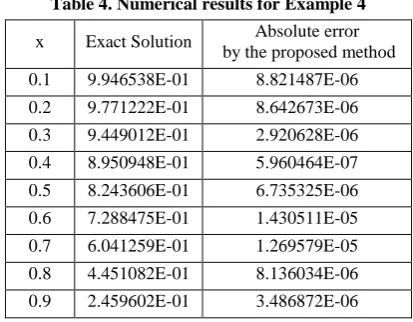
(1-x)ex. The proposed method is tested on this problem where the domain [0,1] is divided into 11 equal subintervals. Numerical results for this problem are shown in Table 4. The maximum absolute error obtained by the proposed method is 1.430511×10⁻⁵.
Table 4. Numerical results for Example 4
x Exact Solution Absolute error by the proposed method 0.1 9.946538E-01 8.821487E-06 0.2 9.771222E-01 8.642673E-06 0.3 9.449012E-01 2.920628E-06 0.4 8.950948E-01 5.960464E-07 0.5 8.243606E-01 6.735325E-06 0.6 7.288475E-01 1.430511E-05 0.7 6.041259E-01 1.269579E-05 0.8 4.451082E-01 8.136034E-06 0.9 2.459602E-01 3.486872E-06
Example 5 Consider the nonlinear boundary value problem
y(10 ) = e-xy2(x), 0<x<1 (33) subject to the boundary conditions
y(0) = 1, y(1) = e, y'(0) = 1, y'(1) = e,
[image:5.595.63.271.505.659.2] [image:5.595.324.531.506.667.2]Volume 51– No.15, August 2012 y'''(0) = 1, y'''(1) = e,
y(4)(0) = 1, y(4)(1) =e. The exact solution for the above problem is given by y(x) =
ex. This nonlinear boundary value problem is converted into a sequence of linear boundary value problems generated by quasilinearization technique [15] as
y(n+1)(10)+[-2e-xy(n)]y(n+1) = -e-x y(n)2, for n = 0,1,2... (35) subject to the boundary conditions
y(n+1)(0) = 1, y(n+1)(1) = e, y(n+1)'(0) = 1, y(n+1)'(1) = e,
y(n+1)''(0) = 1, y(n+1)''(1) = e, (36) y(n+1)'''(0) = 1, y(n+1)'''(1) = e,
y(n+1)(4)(0) = 1, y(n+1)(4)(1) =e. Here y(n+1) is the (n+1)th approximation for y. The domain [0,
[image:6.595.323.531.149.314.2]1] is divided into 11 equal subintervals and the proposed method is applied to the sequence of problems (35). Numerical results for this problem are presented in Table 5. The maximum absolute error obtained by the proposed method is 6.794930 × 10⁻⁵.
Table 5. Numerical results for Example 5
x Exact Solution Absolute error by the proposed method 0.1 1.105171 1.251698E-05 0.2 1.221403 8.702278E-06 0.3 1.349859 2.145767E-06 0.4 1.491825 1.132488E-05 0.5 1.648721 3.969669E-05 0.6 1.822119 5.400181E-05 0.7 2.013753 6.794930E-05 0.8 2.225541 4.887581E-05 0.9 2.459603 2.002716E-05
Example 6 Consider the nonlinear boundary value problem
y(10 )-y'''= 2ex y2, 0<x<1 (37) subject to the boundary conditions
y(0) = 1, y(1) = 1/e, y'(0) = -1, y'(1) = -1/ e,
y''(0) = 1, y''(1) = 1/e, (38) y'''(0) = -1, y'''(1) = -1/e,
y(4)(0) = 1, y(4)(1) =1/e.
The exact solution for the above problem is given by y(x) = e-x. This nonlinear boundary value problem is converted into a sequence of linear boundary value problems generated by quasilinearization technique [15] as
y(n+1)(10)-y(n+1)''' + [-4exy(n)]y(n+1) = -2ex y(n)2, for n = 0,1,2... (39) subject to the boundary conditions
y(n+1)(0) = 1, y(n+1)(1) =1/ e, y(n+1)'(0) = -1, y(n+1)'(1) = -1/e,
y(n+1)''(0) = 1, y(n+1)''(1) = 1/e, (40) y(n+1)'''(0) = -1, y(n+1)'''(1) = -1/e,
y(n+1)(4)(0) = 1, y(n+1)(4)(1) =1/e.
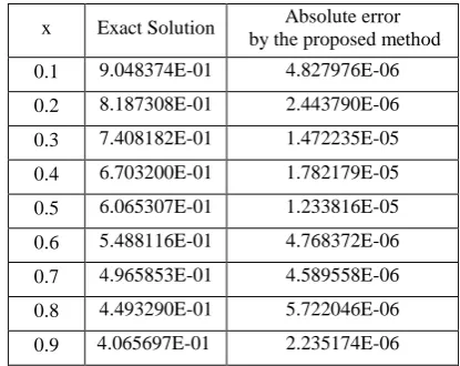
Here y(n+1) is the (n+1)th approximation for y. The domain [0, 1] is divided into 11 equal subintervals and the proposed method is applied to the sequence of problems (39). Numerical results for this problem are presented in Table 6. The maximum absolute error obtained by the proposed method is 1.782179 × 10⁻⁵.
Table 6. Numerical results for Example 6
x Exact Solution Absolute error by the proposed method 0.1 9.048374E-01 4.827976E-06 0.2 8.187308E-01 2.443790E-06 0.3 7.408182E-01 1.472235E-05 0.4 6.703200E-01 1.782179E-05 0.5 6.065307E-01 1.233816E-05 0.6 5.488116E-01 4.768372E-06 0.7 4.965853E-01 4.589558E-06 0.8 4.493290E-01 5.722046E-06 0.9 4.065697E-01 2.235174E-06
Example 7 Consider the nonlinear boundary value problem
4 14175
) 10
(
y (x + y + 1)11, 0<x<1 (41)
subject to the boundary conditions y(0) = 0, y(1) = 0, y'(0) = -1/2, y'(1) = 1,
y''(0) = 1/2, y''(1) = 4, (42) y'''(0) = 3/4, y'''(1) = 12,
y(4)(0) = 3/2, y(4)(1) = 48. The exact solution for the above problem is given by
. 1 2
2 )
(
x
x x
y This nonlinear boundary value
problem is converted into a sequence of linear boundary value problems generated by quasilinearization technique [15] as
) 1 ( 10 ) ( )
10 ( ) 1
( (11)( 1)
4 14175
n n
n x y y
y
1
10
,
)
1
(
4
14175
) ( 10
)
(n
x
y
ny
x
for n = 0,1,2... (43) subject to the boundary conditions
y(n+1)(0) = 0, y(n+1)(1) = 0, y(n+1)'(0) = -1/2, y(n+1)'(1) = 1,
y(n+1)''(0) = 1/2, y(n+1)''(1) = 4, (44) y (n+1)'''(0) = 3/4, y(n+1)'''(1) = 12,
y(n+1) (4)
(0) = 3/2, y(n+1) (4)
(1) = 48.
Table 7. Numerical results for Example 7
x Exact Solution Absolute error by the proposed method 0.1 -4.736842E-02 1.322478E-06 0.2 -8.888889E-02 4.231930E-06 0.3 -1.235294E-01 1.676381E-05 0.4 -1.500000E-01 4.245341E-05 0.5 -1.666667E-01 6.663799E-05 0.6 -1.714286E-01 6.940961E-05 0.7 -1.615385E-01 4.750490E-05 0.8 -1.333333E-01 1.643598E-05 0.9 -8.181816E-02 2.607703E-07
7. CONCLUSIONS
In this paper, we have developed a collocation method with quintic B-splines as basis functions to solve tenth order boundary value problems. Here we have taken internal mesh points x3, x4, …, xn-3 as the selected collocation points. The quintic B-spline basis set has been redefined into a new set of basis functions which in number match with the number of selected collocation points. The proposed method is applied to solve several number of linear and non-linear problems to test the efficiency of the method. The numerical results obtained by the proposed method are in good agreement with the exact solutions available in the literature. The objective of this paper is to present a simple method to solve a tenth order boundary value problem and its easiness for implementation.
8. REFERENCES
[1] Chandrasekhar. S, 1961, Hydro dynamic and Hydro magnetic Stability, Clarendon Press, Oxford, (Reprinted: Dover Books, New York. 1981) .
[2] Agarwal. R.P, 1986, Boundary Value Problems for higher-order differential equations, World Scientific, Singapore. [3] Twizell. E.H, Boutayeb. A, Djidjeli. K. “Numerical methods for eighth, tenth and twelfth-order eigenvalue problems arising in thermal instability”. Adv. Comput. Math. 2(1994): 407-436.
[4] Siddiqi. S.S, Twizell. E.H. “Spline solutions of linear tenth-order boundary value problems”. International Journal of Computer Mathematics 68(1998): 345-362. [5] Siddiqi. S.S, Akram. G. “Solution of tenth-order boundary
value problems using nonpolynomial spline technique”. International Journal of Applied Mathematics and Computation 190(2007): 641-651.
[6] Siddiqi. S.S, Akram. G. “Solution of tenth-order boundary value problems using eleventh degree spline”.
International Journal of Applied Mathematics and Computation 165(2007): 115-127.
[7] Erturk. V.S, Momani. S. “A reliable algorithm for solving tenth-order boundary value problems”. Num. Algo. 44(2007): 147-158.
[8] Siddiqi. S.S, Ikram. G, Zaheer. S. “Solution of Tenth Order Boundary Value Problems using Variational Iteration Technique”. J. European Scientific Research 30(2009): 326-347.
[9] Barari. A, Omidvar. M, Najaf. T, Abdoul Ghotbi. T. “Homotopy Perturbation Method for solving tenth order boundary value problems”. International Journal of Mathematics and Computation 3(2009): J09.
[10] Scott. M.R, Watts. H.A. “Computional solution of linear two points bvp via orthonormalization”. SIMA J. Numer. Anel. 165(1977): 40-70.
[11] Scott. M.R, Watts. H.A, 1976, A systematized collection of codes for solving two-point bvps, Numerical methods for differential systems, Academic Press.
[12] Scott Layne Watson. M.R. “Solving spline-collocation approximations to nonlinear two point boundary value problems by a homotopy method”. Appl. Math. Comput. 24(1987): 333-357.
[13] Wazwaz. A.M. “The Modified Adomian Decomposition Method for solving linear and nonlinear boundary value problems of tenth-order and twelfth-order”. International Journal of Nonlinear Sciences and Numerical Simulation 1(2000): 17-24.
[14] Djidjeli. K, Twizell. E.H, Boutayeb. A. “Numerical methods for special nonlinear boundary-value problems of order 2m”. Journal of Computational and Applied Mathematics 47(1993): 35-45.
[15] Bellman. R.E, Kalaba. R.E, 1965, Qusilinearization and Nonlinear Boundary value problems, American Elsevier, New York.
[16] Reddy. J.N, 2005, An introduction to the Finite Element Method, 3rd Edition, Tata Mc-GrawHill Publishing Company ltd., New Delhi.
[17] Prenter. P.M, 1989, Splines and Variational Methods, John-Wiley and Sons, New York.
[18] Carl de Boor, 1978, A Practical Guide to Splines, Springer-Verlag.