Model predictive control using fuzzy
decision functions
da Costa Sousa, JM and Kaymak, U
Title
Model predictive control using fuzzy decision functions
Authors
da Costa Sousa, JM and Kaymak, U
Type
Article
URL
This version is available at: http://usir.salford.ac.uk/1818/
Published Date
2001
USIR is a digital collection of the research output of the University of Salford. Where copyright
permits, full text material held in the repository is made freely available online and can be read,
downloaded and copied for noncommercial private study or research purposes. Please check the
manuscript for any further copyright restrictions.
Model Predictive Control Using Fuzzy Decision
Functions
João Miguel da Costa Sousa, Member, IEEE, and Uzay Kaymak, Member, IEEE
Abstract—Fuzzy predictive control integrates conventional
model predictive control with techniques from fuzzy multicriteria decision making, translating the goals and the constraints to pre-dictive control in a transparent way. The information regarding the (fuzzy) goals and the (fuzzy) constraints of the control problem is combined by using a decision function from the theory of fuzzy sets. This paper investigates the use of fuzzy decision making (FDM) in model predictive control (MPC), and compares the results to those obtained from conventional MPC. Attention is also paid to the choice of aggregation operators for fuzzy decision making in control. Experiments on a nonminimum phase, unstable linear system, and on an air-conditioning system with nonlinear dynamics are studied. It is shown that the performance of the model predictive controller can be improved by the use of fuzzy criteria in a fuzzy decision making framework.
Index Terms—Fuzzy criteria, fuzzy decision making (FDM),
fuzzy predictive control, model predictive control (MPC).
I. INTRODUCTION
H
UMAN operators can control complex, nonlinear, and partially unknown systems across a wide range of operating conditions for which conventional linear control techniques often fail or can only be applied locally. Fuzzy logic control (FLC) is one of the most popular techniques for translating human knowledge to control, and has been successfully applied to a large number of consumer products and industrial processes [1]–[3]. Most of these applications of fuzzy control use the approach introduced in the 1970s by Mamdani [4]. The operator’s knowledge is verbalized as a collection of if-then control rules, which are directly translated into a control algorithm.Besides direct fuzzy control, in which the control law is ex-plicitly described by if-then rules, human expertise can be used to define the design specifications. These specifications are translated to performance criteria using fuzzy sets, by defining the (fuzzy) goals and the (fuzzy) constraints for the system under control. This procedure is a particular approach of fuzzy model-based control, following closely the classical model predictive control (MPC) design approach, but it makes use of the fuzzy sets theory in a higher level than in FLC, where the fuzzy rules to control the system are given directly from expert knowledge. In this approach, the appropriate control actions
Manuscript received April 11, 1999; revised April 16, 2000 and August 21, 2000. This paper was recommended by Associate Editor T. Sudkamp.
J. M. da Costa Sousa is with the Department of Mechanical Engineering/ GCAR, Technical University of Lisbon, Instituto Superior Técnico, 1049-001 Lisbon, Portugal (e-mail: [email protected]).
U. Kaymak is with Erasmus University, 3062 PA Rotterdam, The Nether-lands.
Publisher Item Identifier S 1083-4419(01)00089-9.
are obtained by means of a multistage fuzzy decision making (FDM) algorithm, as introduced by Bellman and Zadeh [5]. A mixture of these two approaches constitutes the first applica-tion in this field: automatic train operaapplica-tion using a linguistic description of the system [6]. A different approach called fuzzy multiobjective optimal control is presented in [7], but it is quite complex and difficult to implement in real time. More recently, satisficing decisions have also been used in a similar setting to design controllers [8]. A good survey on model-based approach to fuzzy control and decision making is presented by Kacprzyk [9]. However, in this book only open-loop control applications are reported. This paper undertakes to present the first step in generalizing fuzzy predictive control as MPC with fuzzy decision functions, using the FDM approach to select proper control actions. This procedure can be applied to real-time problems with relatively small sampling times.
This paper begins by describing the application of FDM to control in Section II. Fuzzy goals, fuzzy constraints, and fuzzy decision are presented, and an approach to solve the optimiza-tion problem for fuzzy criteria defined in different sets is pro-posed. Note that FDM applied to control considers multistage FDM. Section III presents possible types of fuzzy objective func-tions for predictive control, discussing briefly the operators to ag-gregate fuzzy criteria. Two illustrative examples are presented in Section IV, where the main features of fuzzy decision functions applied to MPC are shown. The paper ends up with some con-cluding remarks about the presented approach in Section V.
II. FUZZYDECISIONMAKING INCONTROL
Although distinct, it is common to present multistage deci-sion making and FDM in control as synonymous. In fact, the decision problem is more general, and also multistage decision making can be applied to other fields. This paper considers mul-tistage decision making applied to control, similar to the ap-proach taken before by several authors [5], [9]. Note that while the notation used in this section is convenient for control ap-proaches, multistage FDM maintains its generality. When mul-tistage decision making is translated to the control environment, the set of alternatives constitute the different control actions, the
system under control is a relationship between the system inputs
and outputs (or causes and effects), and the mapping relating the inputs to the outputs of the system under control is referred to as the model. Moreover, fuzzy constraints are defined for sev-eral variables presented in the system, which can be “hard” or “soft” constraints, and the decision criteria (fuzzy goals and con-straints) are the translation of the control performance criteria to the decision making setting.
One of the main issues in MPC is the type of model of the system under control [10]. In general, the most utilized types of models are deterministic, stochastic, and/or fuzzy. Another im-portant issue in FDM applied to control is the termination time, which is a generalization of the prediction horizon defined for MPC[11]. A short summary of the different termination times, and possible solutions found in the literature for the the different types of models is presented in the following. A survey with complete references can be found in [9].
• Fixed and predetermined specification time—For deter-ministic models, solutions using dynamic programming, branch-and-bound techniques, genetic algorithms, or neural networks have been proposed. For stochastic models two different formulations are usually employed: maximizing the probability of satisfying fuzzy goals and fuzzy constraints, or maximizing the expected value of the fuzzy decision. For fuzzy models, solutions using dynamic programming, branch-and-bound, interpolative reasoning, and genetic algorithms have been proposed. • Implicitly specified termination time—In these systems,
the process terminates when the outputs reach prespecified values. Only solutions for deterministic models were pro-posed, using graph-theoretic analysis and a branch-and-bound algorithm.
• Fuzzy termination time—It is sometimes useful to con-sider a “softer” definition of the termination time, by allowing its formulation as a fuzzy set, as it was first proposed by Fung [12]. For deterministic, stochastic, or fuzzy models, solutions using dynamic programming or branch-and-bound are possible.
• Infinite termination time—This type of termination time is used for processes whose inputs vary little over a very long time range. Optimal control is sought for these types of processes.
Note that all the solutions proposed are obtained for open-loop control, which hampers the application of the proposed solu-tions for low and medium levels of control in real time. For ex-ample, Kacprzyk [9] states
“We consider open-loop control. Unfortunately,
not much is known about closed-loop (feedback) control in a fuzzy environment in the optimal control-type [5] setting
.”
This paper addresses this shortcoming in the literature, and it considers multistage decision making (control) in a fuzzy envi-ronment considering any type of model in closed-loop control. It assumes that the termination time is fixed and is specified be-forehand. As the formulation is done in an MPC environment, this termination time is the prediction horizon, which is shifted when time evolves. This condition is necessary to allow the ap-plication of multistage FDM to MPC in real time.
In the following, Section II-A presents the definition of fuzzy goals and constraints in the control environment. The aggrega-tion of the different criteria for control applicaaggrega-tions is presented in Section II-B, where the set of possible alternatives is dis-cretized in order to find the optimal control actions. The appli-cation of FDM to predictive control is presented in Section II-C.
A. Fuzzy Goals and Fuzzy Constraints in the Control Environment
Let , with , be a fuzzy goal characterized by its membership function , which is a mapping from the space of the goal to the interval . Let also
be a fuzzy constraint characterized by its membership function , mapping the space of the constraint to the same in-terval . The fuzzy goals and the fuzzy constraints can be defined for the domain of the control actions, system’s outputs, state variables, or for any other convenient domain. Note that fuzzy constraints are usually defined in the domain of the control actions, and fuzzy goals are usually defined in the domain of the state space variables. Initially, FDM in control was applied to systems with discrete states and a finite number of possible transitions between the states, and subsequently it has been extended to systems with continuous states [13]. The fuzzy goals and constraints are then all defined on the set of alternatives. The reasoning applied in this paper for FDM in control allows the combination of goals and constraints from different spaces.
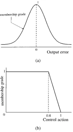
A fuzzy set in the appropriate domain characterizes both the fuzzy goals and the fuzzy constraints. The goals and con-straints are defined on relevant system variables. For example, a common control goal is the minimization of the output error. The satisfaction of this goal is represented by a membership function, which is defined on the space (universe of discourse) of the output error. An example is the fuzzy goal “small output error,” defined for a SISO system and shown in Fig. 1(a). Fuzzy constraints can be defined on the universe of discourse of the control variables. An example is the ‘soft’ constraint “ should not be substantially larger than 0.8,” whose degree of satisfaction can be represented by a membership function, as shown in Fig. 1(b). Note that the “hard” constraint
is also implied by the given membership function. The given examples of a goal and a constraint show that it is sometimes advantageous to treat them in different ways, contrary to the Bellman and Zadeh approach [5].
The qualitative distinction between goals and constraints can be clarified when membership functions for a fuzzy criterion are defined. In this paper, a fuzzy goal is defined in such a way that the membership grade is never zero, unless this is strictly necessary (which would imply that it is a “hard” constraint). Therefore, the example in Fig. 1(a) uses a membership func-tion of the exponential type, which never becomes zero even if the error is quite large. On the other hand, fuzzy constraints must include the “hard” constraints, when they are present in the system. For instance, the constraint in Fig. 1(b) does not allow that the control action is outside the range , which can be a very useful concept for many real systems. Suppose that the variable in Fig. 1(b) is a valve opening, where 1 stands for completely open and 0 for completely closed. Hence, the defi-nition of the fuzzy constraint, as given in Fig. 1(b), takes these physical limitations into account. It is suggested that a fuzzy
con-straint should also represent the “hard” concon-straints when they
(a)
[image:4.612.103.230.62.291.2](b)
Fig. 1. Example of a fuzzy goal and a fuzzy constraint for FDM in control.
distinguishes goals and constraints in the form of the defined membership functions, but clearly does not affect the conflu-ence of criteria.
Assuming as before that one considers goals
and constraints , each fuzzy goal and each fuzzy constraint constitute a decision criterion , where is the total number of goals and constraints. Each criterion is defined in the domain , which can be any of the various domains used in control. In order to solve the problem in reasonable low time, it is defined in a discrete control space with a finite number of control alterna-tives. This limitation to digital control is however not too severe, and this methodology can still be applied to a large number of control problems. Therefore, the confluence of goals and con-straints is defined in the following for discrete alternatives. The resulting optimization problem is also addressed.
B. Aggregation of Criteria in the Control Environment
Assume that a policy is defined as a sequence of control actions for the entire prediction horizon in MPC,
(1) where the control actions belong to a set of alternatives . In the general case, all the criteria must be applied at each time step , with . Thus, a criterion denotes that the crite-rion is considered at time step , with and . Further, let denote the membership value that represents the satisfaction of the decision criteria after applying the control actions . The total number of decision cri-teria for the decision problem is thus given by . The confluence of goals and constraints can be done by aggregating the membership values . The membership value for the
control sequence is obtained using the aggregation operators ,and to combine the decision criteria, i.e.,
(2) In (2), denotes an aggregation operator for combining the goals, denotes an aggregation operator for combining the constraints, and denotes an aggregation operator to combine the aggregated goals and constraints. In general, it is not neces-sary to use the same aggregation operator for all goals and for all constraints. However, using a single aggregation operator re-duces complexity, making the confluence of criteria simpler.
Note that the aggregation operator to combine a goal and a constraint at different time steps, i.e., to
, is the same as the one to combine a goal and a constraint at the same time step, i.e., to
. Various types of aggregation operations can be used as decision functions for expressing different decision strategies using the well-known properties of these operators [14]. In fact, aggregation operators and membership functions translate a lin-guistic description of the control goals into a decision function. In this way, various forms of aggregation can be chosen giving greater flexibility for expressing the control goals. A discussion on the influence of aggregation operators in FDM applied to control is given in Section III-A.
The translation of each goal and each constraint for a given policy to a membership value (2) avoids the specification of the criteria in a large dimensional space. The combination of cri-teria in different domains is done for a set of discrete alternatives, which corresponds to different policies that can be applied to find the optimal control policy. The decision criteria (2) should be satisfied as much as possible, which corresponds to the max-imal value of the overall decision. Thus, the optmax-imal sequence of control actions is found by the maximization of
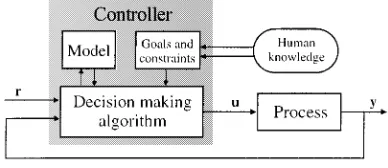
Fig. 2. Controller based on objective evaluation and FDM.
C. Fuzzy Criteria in MPC
The definition of fuzzy goals and constraints must be given by an operator or design engineer. Therefore, when FDM in control is considered, human knowledge is involved in specifying the control objectives and constraints, rather than the control pro-tocol itself [20], [21]. Using a process model, a FDM algorithm selects the control actions that best meet the specifications (see Fig. 2). Hence, a control strategy can be obtained that is able to push the process closer to the constraints, and that is able to force the process to a better performance based on the goals and the constraints set by the operator together with the known con-ditions provided by the system’s designers.
This approach is closely related to MPC. The formulation of the control problem as a confluence of fuzzy goals and fuzzy constraints leads to a generalization of the objective function used in MPC [22]. For practical reasons, it is desirable to have direct control over the influence of the individual components of the objective function on the controller performance. Thus, it is advantageous that the degree of compensation among the different goals and constraints can be specified by the designer. This additional freedom can be achieved by choosing a different representation of the objective function, given by the combina-tion of fuzzy goals and fuzzy constraints, as in the FDM ap-proach. In the MPC environment, a policy with the possible control actions can be defined (1). The objective function using fuzzy criteria is defined (2). The closed-loop control configuration is now discussed in more de-tail, in aspects concerning the criteria and the aggregation oper-ator(s) used to combine them.
III. FUZZYCRITERIA FORFDMINCONTROL
Fuzzy criteria play a main role in FDM. When FDM is ap-plied to control, the fuzzy goals and the fuzzy constraints must be a translation of the (fuzzy) performance criteria defined for the system. The definition of performance criteria in the time domain has shown to be quite powerful, especially for non-linear systems [23] and in the MPC framework [24]. This sec-tion investigates the use of fuzzy performance criteria in pre-dictive control and compares the results to those obtained from conventional MPC. This section is an extension of an introduc-tory study of this subject presented by the authors [25]. First, the aspects concerning the aggregation operator(s) combining the criteria are briefly presented in Section III-A. Next, control criteria and decision functions are discussed in Section III-B, where classical objective functions and a proposed fuzzy objec-tive function are presented.
A. Aggregation Operators for FDM in Control
This section presents some clues on the possible use of dif-ferent aggregation operators, and the advantages and the disad-vantages of their use in predictive control.
The first operator used to aggregate goals and constraints was the minimum operator [5]. In this approach, the operators
, and are all substituted by the minimum operator (2), leading to
(4) Although this operator is still largely used in FDM, it does not allow for any tradeoff or compensation between the criteria, because it chooses always the smallest of the values as the decision. For this reason, this operator is usually known as a safety-first or pessimistic operator. This disadvantage can be overcome by the use of another -norm, which should still trans-late the aggregation as a simultaneous satisfaction of the fuzzy criteria, but allows for some interaction amongst the criteria. The most used aggregation operator after the minimum oper-ator is possibly the product -norm
(5) This operator allows some interaction between the criteria, but keeps the characteristics of -norms, i.e., any low degree of membership for one criteria implies that the degree of mem-bership is also low. When the number of criteria increases, tends to decrease. This fact is quite realistic because the larger the number of goals and constraints is, the more difficult it is to satisfy them all. A similar conclusion can also be drawn for many other -norms.
The presented aggregation operators assume that the importance of different criteria is equal. The attribution of different weights for different criteria can be made by using the weighted-sum in a similar way as it is usually done for classical criteria in predictive control, as will be presented (8). Another possibility is to use the approach presented by Yager [26], where each criterion has a different weight , re-flecting a different importance in the global criterion (2). Other weighted aggregation methods can also be used [14], [27]. In this paper the weights of the aggregation of fuzzy goals and constraints are not used because the systems used as examples do not have a clear hierarchy related to the importance of the different fuzzy criteria. Moreover, the weights can be difficult to tune, especially if a large number of criteria is considered, although they provide additional flexibility to a controller if a good set of tuned weight factors are determined [28].
such as the ones introduced in [29]–[31] and [32]. The Yager -norm, for instance, is given by
(6) with . This operator covers the entire range of -norms, i.e., it goes from the drastic intersection to the minimum oper-ator.
There is a large range of fuzzy operators between the -norms and -norms which can sometimes be advantageously utilized in the confluence of fuzzy criteria for control applications. Exam-ples are the aggregation operator introduced by Zimmermann [33], or the generalized mean [34], [35]. This last operator is given by
(7) It reduces to the harmonic, geometric, arithmetic, and quadratic mean when the parameter is
and , respectively. Moreover, when the generalized mean approaches the minimum operator, and when it approaches the maximum operator. Thus, this op-erator fulfills the complete range from minimum to maximum when ranges from to . When a large number of criteria is present and some tradeoff between the different cri-teria is allowed, this operator can have some advantages over aggregation operators described by -norms. It should be em-phasized, however, that the use of this operator may lead to the violation of “hard” constraints, when they are defined as in Sec-tion II-A. Therefore, when this operator is used, the optimal al-ternative found should be checked afterwards in order to assure that no “hard” constraints are violated. However, this procedure can cost precious optimization time. A solution is to use the gen-eralized mean only for the general confluence operator and a -norm for the remaining and . This choice assures that the “hard” constraints are not violated but can hamper the ad-vantages of using the generalized mean.
This paper uses parameterized operators, and their choice is strongly recommended because they allow for different degrees of compensation between criteria. Moreover, the change of a single parameter results in the use of different operators, alle-viating the tuning phase, always present in predictive control. Section IV-B presents a simple, though illustrative example, showing the application of three different aggregation operators.
B. Control Criteria and Decision Functions
When a control system is designed, performance criteria must be specified. In the time domain, these criteria are usually de-fined in terms of a desired steady-state error between the refer-ence and the output, rise time, overshoot, settling time, etc., rep-resenting the goals of the control system. In MPC, these goals must be translated into an objective function. This function is maximized (or minimized) over the prediction horizon, given the desired control actions. The translation of the (fuzzy) goals into an objective function can be done in two different ways.
• The control goals are explicitly expressed in the objective function. This method leads usually to long term predic-tions of the behavior of the system, using a large prediction horizon . From these predictions, quantities such as the overshoot or the rise time can be determined. In order to have accurate predictions, this method requires a highly accurate process model, which may not be available, and a lot of computation.
• Only short-term predictions (a few steps ahead) are used in the objective function. This method is usually applied in predictive control when the available model of the system is not very accurate, and cannot predict outputs for a large number of steps ahead. Despite this inaccuracy of the model, it still can lead to high-performance control, provided that the overall control goals can be translated into the short-term goals, which are then represented in the objective function. This translation is, however, not unique, and it is application dependent. Therefore, tuning some parameters in the objective function is usually required. This method is especially suitable for nonlinear systems, where a compromise between computational time to derive the control actions and accuracy of the predictions must be made except for special cases, as when input–output (I/O) feedback linearization is utilized [36]. When using fuzzy criteria, the task of defining the goals becomes easier, as it will be shown in this section.
1) Classical Objective Functions: Conventional MPC mainly utilizes sum-quadratic functions as the objective function [11], [37], [38]. The main motivation for its use is that such an objective function has an analytical solution for linear systems without constraints. In the presence of crisp and convex constraints, the optimization problem remains convex for linear systems, and can still be solved in polynomial time. However, the presence of nonconvex constraints and/or the presence of nonlinearities in the system often lead to nonconvex optimization problems. In these cases, the sum-quadratic ob-jective function does not have any advantages over other more complex objective functions that can possibly describe better the (fuzzy) performance criteria for a broad class of control problems.
Let the overall control goals for the time domain be stated as achieving a fast system response while reducing the overshoot and the control effort. For SISO systems these goals can be rep-resented by the objective function
(8) where denotes the predicted errors given by the differ-ence between the referdiffer-ence and the output of the system , i.e., (9) The change of the predicted output is defined as
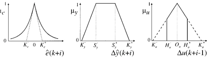
Fig. 3. Membership functions that represent the satisfaction of decision criteria for the error, change in output, and change in the control action.
and is equal to the change in the errors , when the reference to be followed is constant. The change in the control actions is defined in a similar way as
(11) The parameters and are weighting terms that are ap-plication dependent. The parameters and must be selected appropriately depending on the application, and they must satisfy . Usually, , and are chosen equal to one, and equal to , and equal to . Note that the weighting terms
and must reflect the difference of magnitude between the different inputs and/or outputs of the system at various time instants. If this is not the case, and the weights are chosen all equal, for instance, the optimization automatically weights dif-ferent variables, which is not desirable, and it leads to poor con-trol performance.
The objective function (8) can be interpreted as follows. The term containing the predicted errors indicates that these should be minimized, while the term containing the change in the con-trol actions indicates that the concon-trol effort should be reduced. Finally, the term containing the change in the outputs indicates that the system’s output should not suffer sudden changes and, thus, it helps to improve the smoothness of the response. For step references, the change of the output is also equal to the change in the respective output errors except for the discontinuities in the reference signal. Hence, minimizing the output errors and the change of output errors can be regarded as forcing the system to the origin (steady-state solution) in the phase space. The parameters containing the weights, and , can be changed so that the objective function is modified in order to lead to a desired system response. Notice that these parameters have two functions: 1) they normalize the different outputs and inputs of the system and 2) they vary the importance of the three different terms in the objective function (8) over the time steps.
2) Fuzzy Objective Functions: When fuzzy multicriteria
de-cision making is applied to determine the objective function, ad-ditional flexibility is introduced. Each criterion is described by a fuzzy set, where , stands for the time step , and are the different criteria defined for the considered variables at the same time step. Fuzzy criteria can be described in different ways. The most straightforward and easy way is just to adapt the criteria defined for classical objective functions. A SISO system with a control action and an output is considered. Fig. 3 shows examples of general membership functions that can be used for the error
, for the change in the pre-dicted output , and for the change in the control action
, with .
In this example, the minimization of the output error
is represented by an exponential membership function, given by
(12) This well-known function has the nice property of being tangent to the triangular membership function defined using the param-eters and (see Fig. 3). Another interesting feature of this exponential membership function is that it never reaches the value zero, and the membership value is still quite consid-erable, 0.37, for an error of or magnitude. Therefore, this criterion is considered to be a fuzzy goal, as explained in Section II-A. This definition of membership function allows for the comparison of the error parameters, and , to the pa-rameters defined for other fuzzy criteria such as the change in output and the change in control actions.
The change in the output can be represented, for example, by a trapezoidal membership function , as shown in Fig. 3. The system can vary with no limitations in the interval . Outside this interval, physical limitations can be de-fined such that the change in the output can not go below or above . This fuzzy constraint can be seen as a fuzzy goal if no physical limitations are present in the system, and it is not compulsory that the membership value is zero outside a given interval. Note that if this is the case, and can play the same role as and in the membership function defined for the error in (12). Thus, outside the interval expo-nential membership functions as the one defined for the error
can also be used.
be defined as a trapezoidal membership function in a similar way to the one defined for the change in the output.
In principle, different criteria can be defined at each time in-stant . This example has decision criteria (for and ), and the total number of criteria in a fuzzy MPC problem is, thus, given by . Beyond the possibility of defining different criteria for different time steps, it is possible to skip some criteria at certain steps. An example of different criteria at different time steps can be the spread of the membership function defined for the error, which can be nar-rowed as the time approaches , i.e., it is more important to achieve the goal of small error close to the prediction horizon. This corresponds to a decreasing value of in Fig. 3. Some-times it is also advantageous to consider some criteria just at a particular time step. One example is the variation of the con-trol action, which can be quite small for steady-states, but it should change quite significantly for different situations, e.g., when a step response must be followed. The designer should, thus, choose carefully the criteria at each time step, regarding the desired performance criteria of the system under control. In general, all the parameters of the different membership func-tions are application dependent. However, it is possible to derive some tuning guidelines, as will be described in Section IV.
The membership functions quantify how much the system satisfies the criteria given a particular control sequence, bringing various quantities into a unified domain. The use of the membership functions introduces additional flexibility for ex-pressing the control goals, and it leads to increased transparency as it becomes possible to specify explicitly what type of system response is desired. For instance, it becomes easier to penalize errors that are larger than a specified threshold more severely. Note that there is no need to scale the several parameters
and as in (8) when fuzzy objective functions are used, because the use of membership functions introduce directly the normalization required. For this particular aspect, this feature reduces the effort on designing MPC with fuzzy objective functions, when compared to classical objective functions.
After the membership functions have been defined, they are combined by using a decision function, such as a para-metric aggregation operator from the fuzzy sets theory (see Section III-A).
IV. APPLICATIONEXAMPLES
This section presents two simulation examples showing the influence of the conventional and the fuzzy objective functions in predictive control. After the description of the systems, the choice of aggregation operators is discussed for one of the sys-tems. Next, classical and fuzzy objective functions are applied to the systems, and a discussion over the obtained results is made. Other applications of some aspects of the presented approach can be found in [22] and [28].
A. Description of the Simulated Systems
[image:8.612.311.548.63.241.2]The influence of conventional and fuzzy objective functions in predictive control has been studied using two different sys-tems: 1) a simulated nonminimum phase, open-loop unstable
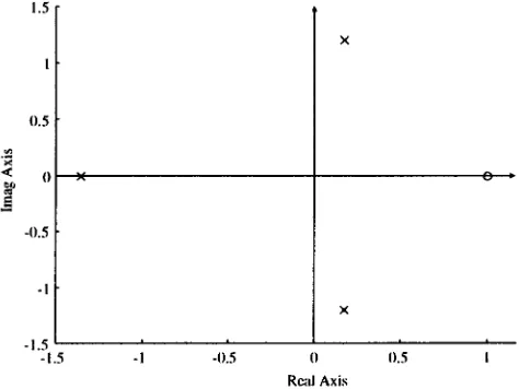
Fig. 4. Position of the poles and zeros of the linear system given by (13).
linear system and 2) a simplified nonlinear model of an air-con-ditioning system, which is derived from real data of a test cell using fuzzy modeling techniques. The following sections de-scribe these systems in more detail. In order to concentrate on the differences between the two control schemes, model-plant mismatch, and the implementational aspects are not considered.
1) Linear System: A linear system has been selected for the
first set of experiments in order to be able to compare the con-trol results when classical and fuzzy criteria are applied. The selected system is described by the transfer function
(13) This is a nonminimum phase system and it has two complex poles in the right-half plane (unstable in open-loop). The poles and zero placement are given in Fig. 4. The system, proceeded by a zero-order-hold circuit, has been discretized with a sample time of one s.
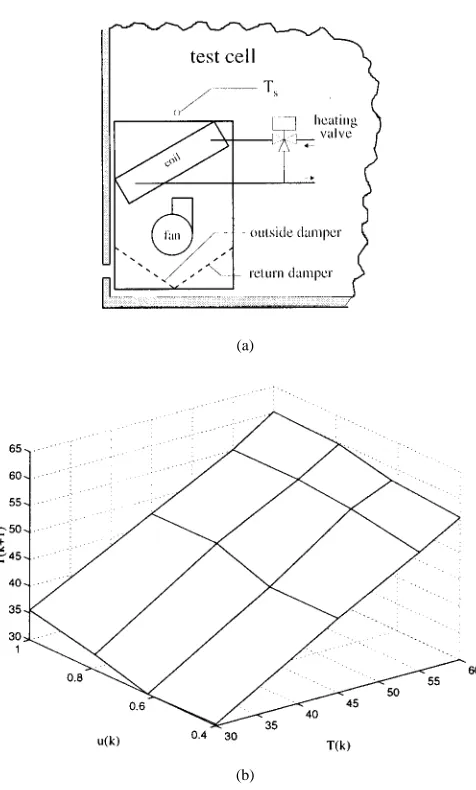
2) Air Conditioning System: A heating, ventilating, and air
(a)
[image:9.612.370.483.62.287.2](b)
Fig. 5. Air conditioning system: (a) schematic representation and (b) derived model.
identification method described in [39]. Fig. 6 shows the trian-gular membership functions that are determined for the temper-ature and the valve opening . Note that the universe of discourse for the valve opening is the interval because the valve shows a dead-zone behavior between 0 and 0.4, when the system is considered to be a SISO system. The fuzzy rule base that describes the model is given in Table I. An example of a rule for this Singleton model, e.g., the first rule, is “If is
Small and is Low, then .”
Fig. 5(b) depicts the piecewise linear mapping that is de-scribed by the fuzzy model. The fuzzy model is used for simu-lating the system and developing predictive controllers.
B. Application of Aggregation Operators to the Linear System
In this section, several issues such as interaction amongst criteria, the influence of the types of decision functions and their parameters are studied using the simulated linear system given in (13). The membership functions for the fuzzy goals and the constraints are assumed to be given. Remember that this system is nonminimum phase and has two complex poles
(a)
[image:9.612.45.283.66.461.2](b)
Fig. 6. Membership functions for the antecedent variables of the fuzzy model. TABLE I
RULEBASE FOR THEFUZZYMODEL OF THEHVAC PROCESS
in the right-half plane (unstable in open loop). Only the mini-mization of the predicted output error is used as optimini-mization criterion in order to keep the optimization problem transparent and to understand clearly the influence of the decision function on the solution. The optimization criterion is represented by a symmetric exponential membership function which is defined around zero output error as
where is the reference and is the predicted model output. This function is a particular case of (12) for . A crisp constraint is imposed on the rate of the control action, and it is represented by a membership function that is defined on .
gen-Fig. 7. Response of a fuzzy predictive controller using the generalized mean as the decision function. Dashed:w = 01, solid: w = 1, dash-dotted: w = 3.
eralized minimum (15), and the Yager -norm (16) are chosen as possible decision functions
(14)
(15)
(16) where , i.e., Zadeh’s fuzzy com-plement. The responses with the parametric decision functions have been calculated for several values of the parameters.
It is known that the minimum operator does not allow interac-tion amongst criteria. It optimizes the worst acinterac-tion in the control sequence and makes sure that it is as good as possible. However, because the system has nonminimum phase behavior, the min-imum operator cannot be used for optimization because every control action except for zero will result in an (initial) increase of the error, decreasing the value of . Hence, the “best” control action will be zero, and the controller will not select another con-trol action. For this reason, a decision function that allows for in-teraction amongst criteria is required for this type of system. For the generalized averaging operator (15), when is chosen very large, the system tries to reach the reference value as soon as pos-sible and shows an overshoot. The system slows down for small values of . A fast response without an overshoot is obtained for equal to one (arithmetic mean). Fig. 7 shows the response of the controlled system for several values of the parameter .
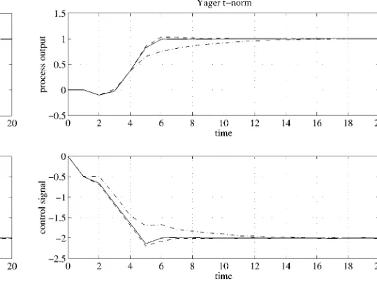
[image:10.612.277.547.63.265.2]Unlike the generalized mean, the system shows fast response for small values of the parameter when the Yager -norm is used. Being a -norm, this operator tries to achieve a simulta-neous satisfaction of all the criteria. The parameter should not be chosen very small as the simultaneous satisfaction of the criteria may then be unfeasible. When is around 2.8, the con-trolled system shows a very fast response without overshoot. The
Fig. 8. Response of a fuzzy predictive controller using the Yagert-norm as the decision function. Dashed:w = 2, solid: w = 2:8, dash-dotted: w = 4.
step response is even faster than the response that is obtained with the arithmetic mean as the decision operator. Fig. 8 shows the step response for several values of . The parameter (or simi-larly the parameter ) can be interpreted as a speed indicator for the response. For small values of , small control actions are preferred and the system response slows down. Large values of favor a faster decrease of the error and, thus, larger control actions are favored. Thus, the system response can be tuned by using the parameter of the decision functions as an extra degree of freedom. Additional objectives such as the rising time and the overshoot could also be controlled with this single parameter.
C. Application of a Fuzzy Objective Function
MPCs have been designed for the systems described in Sec-tion IV-A by using both the convenSec-tional objective funcSec-tion (8) and a fuzzy objective function. A -norm is used for the aggre-gation, since the decision goal is formulated as the simultaneous satisfaction of all the decision criteria. The aggregation opera-tors , and in (2) are taken as the Yager -norm, which combines the control criteria presented in Fig. 3, and is given by
(17) where the parameters and are defined (8), and Zadeh’s complement is defined (16). The parameter allows for the choice of different -norms (see Section III-A).
[image:10.612.57.292.338.443.2]as small as possible, since in practice the model-plant mismatch hampers the use of long horizons.
In this study, the control space is discretized and the optimal control sequence is determined by an enumerative search. The control horizon is chosen equal to two in order to keep the com-putational load low. To further reduce the comcom-putational load, a two-step optimization approach is used, where a rough solution is found by using a coarse discretization of the control space, fol-lowed by the calculation of a finer solution around the rough so-lution. Other optimization techniques for nonconvex problems, such as the branch-and-bound or genetic algorithms can also be used [40], [41].
1) Linear System: The predictive control scheme is applied
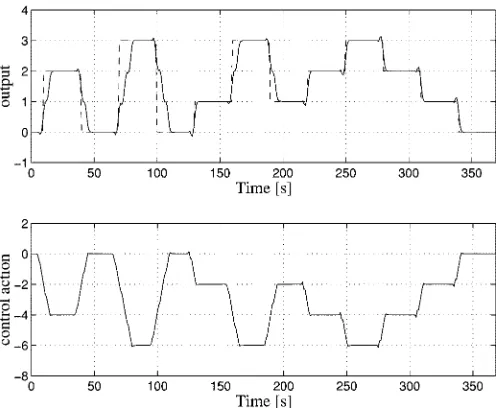
to the linear system given by (13) without any constraints on the system. Both the conventional criteria and the fuzzy criteria are then able to control the system with a fast step response and no overshoot. However, when a rate constraint of
is imposed on the system, the influence of the fuzzy criteria on the control problem becomes more dominant. For these experi-ments, and . It is required that the controller can bring the system to any level in the interval . Using the output error and the change in the output with
[image:11.612.305.552.63.264.2]and was found to be sufficient for controlling the system. The following parameters are used for the conventional objective function: . These values are chosen following the general guidelines pre-sented in [11] and [24], and by trial and error until a reasonable response of the system is found. The parameter was a com-promise between fast response (for smaller values) and small or no overshoot (for bigger values). For the fuzzy criteria, the following membership function parameters are found by tuning , and for the Yager -norm. The way to tune the Yager param-eter is discussed in Section III-A. The membership functions for the error and change in error are chosen to have equal magni-tude by choosing , and by taking and symmetrical to and , respectively. Note that the choice of these four parameters requires only the tuning of one of them, because they are all related. Finally, the parameters and are chosen such that the system can move freely to a certain de-gree, and is penalized outside these limits. The criterion on the change of the control action is not considered because it does not introduce any improvement in the control performance of this system. The responses of the system for several steps using classical and fuzzy criteria are shown in Figs. 9 and 10, respec-tively. It is clear that the predictive controller with fuzzy cri-teria can improve the speed of the response considerably, while avoiding overshoots. The response of the controller with con-ventional criteria can be made faster by changing the values of , but this occurs at the expense of amplifying the oscillations due to the nonminimum phase behavior. Another solution can be found by extending the prediction horizon. However, a con-siderable increase of the prediction horizon is required, and this is in general undesired. Hence, this system benefits clearly from the additional flexibility introduced by the fuzzy criteria. More-over, the prediction horizon can be reduced when fuzzy objec-tive functions are used, without deteriorating the control perfor-mance, when proper fuzzy objectives are designed.
Fig. 9. Step responses for the linear system using the conventional objective function.
Fig. 10. Step responses for the linear system using the fuzzy objective function.
2) Air-Conditioning System: The air-conditioning system
is simulated and a rate constraint of is imposed on the system in these experiments. In this system is chosen equal to two, and is chosen equal to three. These horizons revealed to be sufficient for controlling the system. It is re-quired that the controller can bring the system to any level in the interval [30 C, 60 C], which is the interval where the temperatures usually range for this system. The output error with , the change in the control action with
and the change in the output with
[image:11.612.303.552.316.520.2]the objective function imposes a soft constraint on the change of the second control action, which reduces the oscillations of the control signal without slowing down the response of the system. The output error and the change in output are just considered for the final step , because it requires less control effort in the system. Moreover, the use of the two first steps deteriorates the control performance due to the severe nonminimum phase behavior detected at some regions of the system’s response.
The following parameters are used for the conventional ob-jective function: and . The rest of the parameters are zero. The parameters and are chosen to make a tradeoff between the several criteria, and to scale the different terms: error, change in control action and change in the output. Note that the fuzzy objective function does not require this scaling due to the normalization introduced by the fuzzy sets. For the fuzzy criteria, the following membership function parameters are used:
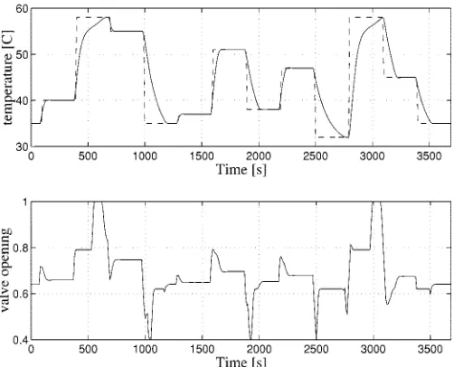
, and . Although nine parameters are present, only five must be tuned because the others are related to them. The parameter is chosen as the maximum error allowed for the system. is the max-imum change allowed in the output. must be smaller than , and this is the region where the temperature can change without being penalized. The parameter is chosen such that the valve can change almost freely (the total range is the in-terval ), because the valve in the real system can change in this way, and the constraint in this valve is made for energy saving and stability reasons. Finally, the parameter for the Yager -norm, , allows for a good compromise between fast response and small overshoot, see Section III-A. The responses of the air-conditioning system for several steps using classical and fuzzy criteria are shown in Figs. 11 and 12, respectively. The controller with the fuzzy criteria is more able to use the full range of control actions, and the response of this controller is in general faster, especially for references close to the limits of the range within which they can vary. Further, some overshoots that are noticeable with the conventional criteria are reduced.
Summarizing, for the studied systems, the use of fuzzy cri-teria improves the response of the predictive controller when the parameters of the objective functions are tuned in order to obtain fast system response without overshoot. Despite the additional number of parameters, tuning the fuzzy criteria is not more te-dious than tuning the conventional objective function because of a better understanding of the influence of the various param-eters. The main disadvantage of the MPC with fuzzy criteria is that the optimization problem often becomes nonconvex, in-creasing then the computational load.
V. CONCLUDINGREMARKS
[image:12.612.303.555.69.272.2]The application of FDM to predictive control in closed-loop control systems is considered in this paper. FDM in control has two main design problems, which are the choice of the ag-gregation operators and the choice of fuzzy criteria. The use of parameterized aggregation operators has some advantages, because these parameters can influence several criteria at the same time. The relation amongst various performance criteria such as the rise time, the settling time or the overshoot can then be adapted with only one parameter. Contrary to many
Fig. 11. Step responses for the air-conditioning system using the conventional objective function.
Fig. 12. Step responses for the air-conditioning system using the fuzzy objective function.
[image:12.612.304.555.320.523.2]Future research must consider the generalization of the fuzzy objective function in order to include weights and hierarchical fuzzy criteria. The methods dealing with the nonconvex opti-mization problem to be solved at each step in MPC need to be computationally efficient. Such methods should be devel-oped and tested in the future, including, e.g., genetic algorithms, branch-and-bound, allowing the application of fuzzy MPC to systems with smaller sampling times.
REFERENCES
[1] T. Terano, K. Asai, and M. Sugeno, Applied Fuzzy Systems. Boston, MA: Academic, 1994.
[2] J. Yen, R. Langari, and L. A. Zadeh, Industrial Applications of Fuzzy
Logic and Intelligent Systems. Piscataway, NJ: IEEE Press, 1995. [3] H. B. Verbruggen and R. Babu˘ska, Eds., Fuzzy Logic Control: Advances
in Applications, Vol. 23 of World Scientific Series in Robotics and Intel-ligent Systems. Singapore: World Scientific, 1999.
[4] E. H. Mamdani, “Applications of fuzzy algorithms for control of simple dynamic plant,” Proc. Inst. Elect. Eng., vol. 121, pp. 1585–1588, 1974. [5] R. E. Bellman and L. A. Zadeh, “Decision making in a fuzzy
environ-ment,” Manage. Sci., vol. 17, no. 4, pp. 141–164, 1970.
[6] S. Yasunobu and S. Miyamoto, “Automatic train operation system by predictive fuzzy control,” in Industrial Applications of Fuzzy Control, M. Sugeno, Ed. Amsterdam, The Netherlands: North-Holland, 1985, pp. 1–18.
[7] L. M. Jia and X. D. Zhang, “On fuzzy multiobjective optimal control,”
Eng. Appl. Artif. Intell., vol. 2, no. 6, pp. 153–164, 1993.
[8] M. A. Goodrich, W. C. Stirling, and R. L. Frost, “A theory of satisficing decisions and control,” IEEE Trans. Syst., Man, Cybern. A, vol. 28, pp. 763–779, Nov. 1998.
[9] J. Kacprzyk, Multistage Fuzzy Control. New York: Wiley, 1997. [10] J. Richalet, “Industrial applications of model based predictive control,”
Automatica, vol. 29, pp. 1251–1274, 1993.
[11] R. Soeterboek, Predictive Control: A Unified Approach. Englewood Cliffs, NJ: Prentice-Hall, 1992.
[12] L. W. Fung and K. S. Fu, “Characterization of a class of fuzzy optimal control problems,” in Fuzzy Automata and Decision Processes, M. M. Gupta, G. N. Saridis, and B. R. Gaines, Eds. Amsterdam, The Nether-lands: North-Holland, 1977, pp. 209–219.
[13] B. Gluss, “Fuzzy multi-stage decision-making fuzzy state and terminal regulators and their relationship to nonfuzzy quadratic state and terminal regulators,” Int. J. Contr., vol. 17, no. 1, pp. 177–192, 1973.
[14] U. Kaymak, “Fuzzy decision making with control applications,” Ph.D. dissertation, Delft Univ. Technol., Delft, The Netherlands, 1998. [15] J. M. Sousa, U. Kaymak, M. Verhaegen, and H. B. Verbruggen, “Convex
optimization in fuzzy predictive control,” in Proc. 35th IEEE Conf.
De-cision Control, Kobe, Japan, 1996, pp. 2735–2740.
[16] P. E. Gill, W. Murray, and M. H. Wright, Practical Optimization. New York: Academic, 1981.
[17] J. A. Nelder and R. Mead, “A simplex method for function minimiza-tion,” Comput. J., vol. 7, pp. 308–313, 1965.
[18] C. Onnen, R. Babu˘ska, U. Kaymak, J. M. Sousa, H. B. Verbruggen, and R. Isermann, “Genetic algorithms for optimization in predictive con-trol,” Contr. Eng. Practice, vol. 5, no. 10, pp. 1363–1372, 1997. [19] J. M. Sousa, R. Babu˘ska, and H. B. Verbruggen, “Fuzzy predictive
con-trol applied to an air-conditioning system,” Contr. Eng. Practice, vol. 5, no. 10, pp. 1395–1406, 1997.
[20] M. A. Goodrich, W. C. Stirling, and M. Zanaboni, “Model predictive satisficing fuzzy logic control,” IEEE Trans. Fuzzy Syst., vol. 7, pp. 319–332, June 1999.
[21] A. Meiritz, H.-J. Zimmermann, R. Felix, and R. Freund, “Goal-oriented control based on fuzzy decision making,” in Proc. 3rd Eur. Congr. Fuzzy
Intelligent Technologies, Aachen, Germany, Aug. 1995, pp. 82–85.
[22] J. M. Sousa, R. Babu˘ska, P. M. Bruijn, and H. B. Verbruggen, “Compar-ison of conventional and fuzzy predictive control,” in Proc. 1996 IEEE
Int. Conf. Fuzzy Systems, New Orleans, LA, Sept. 1996, pp. 1782–1787.
[23] J. J. E. Slotine and W. Li, Applied Nonlinear Control. Englewood Cliffs, NJ: Prentice-Hall, 1991.
[24] E. F. Camacho and C. Bordons, Model Predictive Control in the Process
Industry. New York: Springer-Verlag, 1995.
[25] U. Kaymak, J. M. Sousa, and H. B. Verbruggen, “A comparative study of fuzzy and conventional criteria in model-based predictive control,” in
Proc. 1997 IEEE Int. Conf. Fuzzy Systems, Barcelona, Spain, July 1997,
pp. 907–914.
[26] R. R. Yager, “On the inclusion of importance in multi-criteria decision making in the fuzzy set framework,” Int. J. Expert Syst., Res. Applicat., vol. 5, pp. 211–228, 1992.
[27] U. Kaymak and H. R. van Nauta Lemke, “A sensitivity analysis approach to introducing weight factors into decision functions in fuzzy multicri-teria decision making,” Fuzzy Sets Syst., vol. 97, no. 2, pp. 169–182, July 1998.
[28] U. Kaymak and J. M. Sousa, “Model based fuzzy predictive control ap-plied to a simulated gantry crane,” in Proc. 2nd Asian Control Conf., vol. 3, Seoul, Korea, July 1997, pp. 455–458.
[29] H. Hamacher, “Über logische verknupfungen unscharfer aussagen und deren zugehörige bewertungsfunktionen,” in Progress in
Cyber-netics and Systems Research, G. J. Klir, R. Trappl, and L. Ricciardi,
Eds. Washington, DC: Hemisphere, 1978.
[30] R. R. Yager, “On a general class of fuzzy connectives,” Fuzzy Sets Syst., vol. 4, pp. 235–242, 1980.
[31] S. Weber, “A general concept of fuzzy connectives, negations and im-plications based ont-norms and t-co-norms,” Fuzzy Sets Syst., vol. 11, pp. 115–134, 1983.
[32] D. Dubois and H. Prade, “New results about properties and semantics of fuzzy set-theoretic operators,” in Fuzzy Sets, P. P. Wang and S. K. Chang, Eds. New York: Plenum, 1986.
[33] H. J. Zimmermann and P. Zysno, “Latent connectives in human decision making,” Fuzzy Sets Syst., vol. 4, pp. 37–51, 1980.
[34] H. R. van Nauta Lemke, J. G. Dijkman, H. van Haeringen, and M. Pleeging, “A characteristic optimism factor in fuzzy decision-making,” in Proc. IFAC Symp. Fuzzy Information, Knowledge Representation,
Decision Analysis, Marseille, France, 1983, pp. 283–288.
[35] U. Kaymak and H. R. van Nauta Lemke, “A parametric generalized goal function for fuzzy decision making with unequally weighted ob-jectives,” in Proc. 2nd IEEE Int. Conf. Fuzzy Systems, vol. 2, Mar. 1993, pp. 1156–1160.
[36] M. A. Henson and D. E. Seborg, “Input-output linearization of general nonlinear systems,” AIChE J., vol. 36, pp. 1753–1757, 1990. [37] D. W. Clarke, C. Mohtadi, and P. S. Tuffs, “Generalized predictive
con-trol. Part 1: The basic algorithm. Part 2: Extensions and interpretations,”
Automatica, vol. 23, no. 2, pp. 137–160, 1987.
[38] D. W. Clarke and C. Mohtadi, “Properties of generalized predictive con-trol,” Automatica, vol. 25, no. 6, pp. 859–875, 1989.
[39] R. Babu˘ska and H. B. Verbruggen, “A new identification method for linguistic fuzzy models,” in Proc. FUZZ, Yokohama, Japan, Mar. 1995, pp. 905–912.
[40] J. M. Sousa, “A fuzzy approach to model-based control,” Ph.D. disser-tation, Delft Univ. Technol., Delft, The Netherlands, Apr. 1998. [41] J. M. Sousa, P. M. Bruijn, and H. B. Verbruggen, “Branch-and-bound
optimization in real-time fuzzy predictive control,” Int J. Intell. Syst., vol. 15, no. 9, pp. 879–899, Oct. 2000.
João Miguel da Costa Sousa (S’96–M’98) was born in 1966 in Lisbon,
Por-tugal. He received the M.Sc. degree in mechanical engineering from the Tech-nical University of Lisbon in 1992 and the Ph.D. degree in electrical engineering from the Delft University of Technology, Delft, The Netherlands, in 1998.
He is currently an Assistant Professor in the Control, Automation, and Robotics Group, Department of Mechanical Engineering, Instituto Superior Técnico, Technical University of Lisbon. His main research interests include fuzzy model-based control, intelligent and predictive control, and fuzzy decision making.
Uzay Kaymak (S’94–M’97) received the M.Sc. degree in electrical engineering
in 1992, the Chartered Designer degree in information technology in 1995, and the Ph.D. degree in 1998 all from Delft University of Technology, Delft, The Netherlands.
From 1997 to 2000, he was a Reservoir Engineer at Shell International Ex-ploration and Production. Currently, he is an Assistant Professor at Erasmus University, Rotterdam, The Netherlands. His current research interests include fuzzy decision making and intelligent marketing and finance.