Delay time modelling
Wang, W
Title
Delay time modelling
Authors
Wang, W
Type
Book Section
URL
This version is available at: http://usir.salford.ac.uk/2546/
Published Date
2008
USIR is a digital collection of the research output of the University of Salford. Where copyright
permits, full text material held in the repository is made freely available online and can be read,
downloaded and copied for noncommercial private study or research purposes. Please check the
manuscript for any further copyright restrictions.
Delay Time Modelling
Wenbin Wang
14.1 Introduction
In this chapter we present a modelling tool that was created to model the problems of inspection maintenance and planned maintenance interventions, namely Delay Time Modelling (DTM). This concept provides a modelling framework readily applicable to a wide class of actual industrial maintenance problems of assets in general, and inspection problems in particular.
The concept of the delay time was first mentioned by Christer in 1976 in a context of building maintenance, Christer (1976). It was not till 1984, the concept was first applied to an industrial maintenance problem, Christer and Waller (1984). Since then, a series of research papers appeared with regard to the theory and applications of delay time modelling of industrial asset inspection problems, see Christer (1999) for a detailed review. The delay time concept itself is simple which defines the failure process of an asset as a two-stage process. The first stage is the normal operating stage from new to the point that a hidden defect has been identified. The second stage is defined as the failure delay time from the point of defect identification to failure. It is the existence of such a failure delay time which provides the opportunity for preventive maintenance to be carried out to remove or rectify the identified defects before failures. With appropriate modelling of the durations of these two stages, optimal inspection intervals can be identified to optimise a criterion function of interest.
DTM provides a rich source of modelling methodologies ranged from the concept to practical solutions.
Asset inspection modelling has long been researched by many others, Among them, the model proposed by Barlow and Proschan (1965) is perhaps the most famous one. They consider a unit subject to inspections as follows. The unit is inspected at prespecified times, where each inspection is executed perfectly and instantaneously. The policy terminates with an inspection which detects the unit failure. This implies that the unit may have already failed during an operation interval between inspections, but can only be identified at the forthcoming inspection. Various modifications and extensions to the Barlow and Proschan’s model have been proposed, see for example, Thomas et al (1991), Luss (1981), Abdel-Hameed (1995), Kaio and Osaki (1989), McCall (1965). The delay time inspection model is different from the classical Barlow and Proschan’s model on two accounts. First, a failure is identified immediately when it occurs. This is perhaps more rationale than the Barlow and Proschan’s model since if the system fails, it may have stopped operating and should be observed immediately by the operators. Secondly, there is a failure delay time in DTM which characterises the abnormal deterioration before failure, which is not defined in Barlow and Proschan’s model. It is noted however, that for a certain class of equipment such as fire distinguishers, Barlow and Proschan ’s model is appropriate.
To clarify the objective of the type of inspection modelling we are concerned with here, consider a plant item with an inspection practice every period T, says, weeks, months, … , with repair of failures undertaken as they arise. The inspection consists of a check list of activities to be undertaken, and a general inspection of the operational state of the plant. Any defect identified leads to immediate repair, and the objective of the inspection is to minimise operational downtime. Other objectives could be considered, for example cost, availability or output. There are other types of inspection activities such as condition monitoring and preventive maintenance which will be introduced and discussed elsewhere in this book, for now we focus on the inspection practice outlined above using the delay time inspection modelling technique.
This chapter is organised as follows. Section 14.2 gives an outline of the delay time concept. Sections 14.3 and 14.4 introduce two delay time inspection models of a single component and a complex system respectively. Section 14.5 discusses the parameters estimation techniques used in DTM. Section 14.6 highlights extensions to the basic delay time model and future research in DTM and section 14.7 concludes the chapter.
14.2 The Delay Time Concept
as an example, the case for a single component will be considered in section 14.3. The interaction between inspection and equipment performance may be captured using the delay time concept presented below.
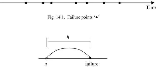
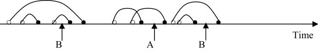
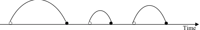
Let the item of an asset be maintained on a breakdown basis. The time history of breakdown or failure events is a random series of points, see Fig. 14.1. For any one of these failures, the likelihood is that, had the item been inspected at some point just prior to failure, it could have revealed a defect which, though the item was still working, would ultimately lead to a failure. Such signals include excessive vibration, unusual noise, excessive heat, surface staining, smell, reduced output, increased quality variability etc. The first instance where the presence of a defect might reasonably be expected to be recognised by an inspection, had it taken place, is called the initial point u of the defect, and the time
h
to failure from u is called the delay time of the defect, see Fig 14.2. Had an inspection taken place in, the presence of a defect could have been noted and corrective actions taken prior to failure. Given that a defect arises, its delay time represents a window of opportunity for preventing a failure. Clearly, the delay time h is a characteristic of the item concerned, the type of defect, the nature of any inspection, and perhaps the person inspecting. For example, if the item was a vehicle, and the maintenance practice was to respond when the driver reported a problem, then there is in effect a form of continuous monitoring inspection of cab related aspects of the vehicle, with a reasonably long delay time consistent with the rate of deterioration of the defect. However, should the exhaust collapse because a support bracket was corroded through, the likely warning period for the driver, the delay time, would be virtually zero, since he would not normally be expected to look under the vehicle. At the same time, had an inspection been undertaken by a service mechanic, the delay time may have been measured in weeks or months. Had the exhaust collapsed because securing bolts became loose before falling out, then the driver could have had a warning period of excessive vibration, and perhaps noise, and the defects would have had a drive related delay time measured in days or weeks.
)
,
(
h
u
+
h
● ● ● ● ● ● ●
[image:4.595.153.460.523.659.2]Time
Fig. 14.1. Failure points ‘●’
○ ● h
u failure
To see why the delay time concept is of use, consider Fig. 14.3 incorporating the same failure point pattern as Fig 14.1 along with the initial points associated with each failure arising under a breakdown system. Had an inspection taken place at point (A), one defect could have been identified and the seven failures could have been reduced to 6. Likewise, had inspection taken place at points (B) and point (A), 4 defects could have been identified and the 7 failures could have been reduced to 3. Fig. 14.3 demonstrats that provided it is possible to model the way defects arise, that is the rate of arrival of defects
λ
(
u
)
, and their associated delay time , then the delay time concept can capture the relationship between the inspection frequency and the number of plant failures.h
We are assuming for now that inspections are perfect, that is, a defect is recognised if it is, and only if it is, there and is removed by corrective action. Delay Time Modelling is still possible if these assumptions are not valid, but this more complex case is discussed in section 14.3.1.
○ ○ ● ○ ● ● ○ ○ ● ● ○○ ● ●
[image:5.595.152.472.347.401.2]B A B Time
Fig. 14.3. ‘○’ initial points; ‘●’ failure points.
14.3 Delay Time Models for Complex Plant
14.3.1 Perfect inspections
A complex plant, or multi-component plant, is one where a large number of failure modes arise, and the correction of one defect or failure has nominal impact in the steady state upon the overall plant failure characteristics. Consider the following basic complex plant maintenance modelling scenario where:
1. An inspection takes place every
T
time units, costs units and requires time units, wheres
c
s
d
ds <<T.2. Inspections are perfect in that all (and only) defects present are identified. 3. Defects identified are repaired during the inspection period.
4. Defects arise according to a Homogeneous Poisson Process (HPP) with the rate of occurrence of defects,
λ
, per unit time.5. The delay time,
H
, of a random defect is described by a pdf. , cdf. , and is independent of the initial pointU
.)
(
h
f
6. Failure will be repaired immediately at an average cost and downtime .
f
c
f
d
7. The plant has operated sufficiently long since new to be considered effectively in a steady state.
8. Defects and failures only arise whilst plant is operating.
These assumptions characterise the simplest non-trivial inspection maintenance problem, Christer et al (1995), and would, of course, only be agreed in any particular case after careful analysis and investigation of the specific situation. We now proceed to construct the mathematical model of the relationship between T and an objective function of interest.
From assumptions 1-4, it is obvious that the number of system failures is identical and independent over each inspection interval, and we can simply study the behaviour of such a failure process over one interval, say the first interval
[
0
,
T
)
. Suppose for now that we take the expected downtime per unit time, , as a measure of our objective function, the relationship between)
(
T
D
T
and can be established directly by using the renewal reward theorem, Ross (1981), as)
(
T
D
[(
( )]
(Downtime over t)
( ) lim
f ft
s
d E N
T
d
E
D T
t
T
→∞
s
d
+
=
=
+
(14.1)where is the expected number of failures within [0,T). Clearly if is available, can be readily calculated.
)]
(
[
N
T
E
f)]
(
[
N
T
E
fD
(
T
)
It can be shown that the failure process shown in Fig. 14.3 is a Marked Poisson process, Taylor and Karlin (1998), with the delay time h as the marker. It has been proved that this failure process over is a nonhomougenous Poisson process (NHPP), Taylor and Karlin (1998) and Christer and Wang (1995). To derive the the rate of occurrence of failures (ROCOF),
)
,
0
[
T
)
(
t
ν
, for this NHPP, within , we start first by deriving the expected number of failures within . Since the expected number of the defects arrived within [)
,
0
[
T
)
,
0
[
T
t
t
t
,
+
δ
),0
≤
t
<
T
, isλδ
t
, then the expected value of the failures caused by these defects isλ
F
(
T
−
t
)
δ
t
. Integrating fromt
0
toT
and after some manipulation we have∫
=
Tf
T
F
t
dt
N
E
0
(
)
)]
(
[
λ
(14.2)Differentiating (14.2) with respect to
T
we have)
(
)
(
t
F
t
The original model developed in Christer and Waller (1984) for (14.2) uses a different approach, but leads to the same result.
14.3.2 Imperfect inspections
Section 14.3.1 outlined a basic delay time model under perfect inspections. It is established under a set of assumptions, and some of them may not be valid in practical situations. These assumptions greatly simplify the mathematics involved but also restrict a wider use of the models developed. Perhaps the most restrictive assumption is that of perfect inspections. In almost all the case studies conducted using the delay time concept, we found none of them supported the perfect inspection assumption. The other concerning assumption is the HPP for defect arrival in the case of a complex system. One would naturally think as the system ages there could be more defect arrivals than that of a younger system. In this section, we introduce one delay time model that relaxes the perfect inspection assumption. The delay time model using a NHPP is presented in Christer and Wang, (1995) and Wang and Christer(2003). These models are mainly developed for complex systems, but a non-perfect inspection single component delay time model can also be developed along a similar line, Baker and Wang (1991).
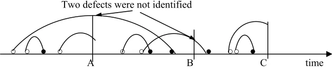
All the assumptions proposed in section 14.3.1 will hold except the perfect inspection one. Assume for now that if a defect is present at an inspection, then there is a probability
r
that the defect can be identified. This implies that there is a probability1
−
r
that the defect will be unnoticed. Fig. 14.4 depicts such a process.Two defects were not identified
[image:7.595.148.472.441.512.2]○ ○ ● ○ ○ ○ ● ● ● ○○ ● A B C time
Fig. 14.4. Failure process of a multi-component system subject to three non-perfect inspections at points A, B, and C, and two potential failures were removed and two missed. It has been proved that the failure process over each inspection interval is still an NHPP, Christer and Wang (1995), but not identical over the earlier inspection intervals of the system. It can be shown that as the number of inspections increases, the number of failures over each inspection interval becomes stable and identical, so we need to study the asymptotic behaviour of the failure process assuming the number of previous inspections is very large.
Let
i
--- th inspection;i
U
--- random variable of the initial time u;r
--- probability of perfect inspection;)
(
t
i)]
,
)
1
((
[
N
i
T
iT
E
f−
--- expected number of failures over[(
i
−
1
)
T
,
iT
)
;)]
(
[
N
iT
E
s --- expected number of defects identified atiT
;It can be shown, Christer et al (1995), Christer and Wang (1995), that is given by
)
(
t
v
i)
)
1
(
(
)]
(
)
)
1
(
(
[
)
1
(
)
(
1 1T
i
t
F
nT
t
F
T
n
t
F
r
t
v
i=
∑
in=−
i n−
−
−
−
+
−
−
+
−
λ
λ
(14.4)for
t
∈
[(
i
−
1
)
T
,
iT
)
.It can also be proved by induction that
v
i−1(
t
)
≈
v
i(
t
)
when i is large. Given(14.4) is available, it is straightforward that the expected number of failures over is given by
)
,
)
1
[(
i
−
T
iT
{
}
∫
∑
∫
− = + − −−
−
+
−
−
−
−
−
=
=
−
iT T i i n n i iT T i i fdt
T
i
t
F
nT
t
F
T
n
t
F
r
dt
t
v
iT
T
i
N
E
) 1 ( 1 1 ) 1 ()
)
1
(
(
)]
(
)
)
1
(
(
[
)
1
(
)
(
)]
,
)
1
((
[
λ
λ
(14.5)The expected number of defects found at an inspection point, say,
iT
, is also a Poisson variable with the mean given by, Christer et al (1995), Christer and Wang (1995)∫
∫
∑
= − − + −−
−
+
−
−
−
=
iT T i nT T n i n n i sdu
u
iT
F
r
du
u
iT
F
r
r
iT
N
E
) 1 ( ) 1 ( 11
[
1
(
)]
[
1
(
)]
)
1
(
)]
(
[
λ
λ
(14.6)The expected downtime is given by (14.1) with the expected numer of failures given by by (14.5), so that
s s f f
d
T
d
T
T
i
N
E
d
T
D
+
+
−
=
[
((
1
)
,
)]
)
(
(14.7)The use of (14.7) assumes that the system is already in a steady state with . For computation purpose we can select a large , and then starts from the first k
where and
∞
→
i
i
n
ε
≥
−
)
− +11
(
i kEquation (14.7) is established assuming that the defects identified at an inspection will always be removed without costing any extra downtime or cost. This assumption can be relaxed. Let be the mean downtime per defect being repaired. Then using the same approach as before, the expected downtime is given by
r
d
)]
(
[
)]
(
[
)]
,
)
1
((
[
)
(
iT
N
E
d
d
T
iT
N
E
d
d
T
T
i
N
E
d
T
D
s r s
s r s f
f
+
+
+
+
−
=
, (14.8)If the objective function is the expected cost per unit time, we obtain this by simply substituting the downtime parameters in (14.7) or (14.8) by the corresponding cost parameters.
Example
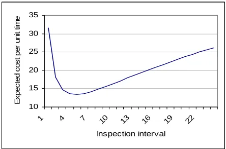
Assume that the rate of occurrence of defects is 2 per day, and the delay time distribution is exponential with scale parameter 0.03 measured in days. The downtime measures are
d
f=
30
andd
s=
30
minutes respectively. Theprobability of a perfect inspection is assumed to be 0.7. Using (14.5) and (14.7), we have the expected downtime against inspection intervals as shown in Fig. 14.5
10 15 20 25 30 35
1 4 7 10 13 16 19 22
Inspection interval
E
x
p
e
c
te
d
co
st p
e
r u
n
it t
im
[image:9.595.186.408.423.570.2]e
Fig. 14.5 Expected downtime per unit time v inspection interval (in days) It can be seen from Fig. 14.5 that a weekly inspection interval is the best.
14.4 Delay Time Model for A Component Subject To A Single
Failure Mode (Single Component System)
are plant items which may have a single dominant failure mode, and may be, in some cases, replaced or renewed upon failure. Examples of such plant items are batteries, traffic lights, small pumps and motors. Such plant items are called single component systems. Noted that a system in this category may not actually be a single component, but the key difference compared with a complex multi-component system is that this single multi-component system is subject to a single failure mode, and the only maintenance action is to renew the whole system either by a complete replacement or a renewal type of repair. This implies that at any point of time, only one defect of the dominant failure mode can exist. This contrasts with a complex system with many failure modes, where only the failed component was replaced or repaired upon a failure, and at any point of time there could be many defects present, and the system is not renewed at failures.
The failure process of this type of a single plant item is different from that of a multi-component complex system, see Figs. 14.6 and 14.7.
○
○
●
○
●
●
○
○
●
●
○○
●
●
Fig. 14.6 Failure process of a multi-component system, where ‘○’ denotes initial
points; ‘●’ failure points.
[image:10.595.150.474.428.477.2]○
●
○
●
○
●
Time Time
Fig. 14.7 Failure process of a single component system
For the system in Fig. 14.6, the system may be renewed at inspection points if these inspections are perfect, and the rate of arrival of defects is constant. However for the system in Fig.14.7, the system can be renewed either at a failure or at an inspection. We present the case with a perfect inspection assumption. The case of an imperfect inspection delay time model for a single component can be found in Baker and Wang (1991), (1993).
We need the following additional assumptions and notation.
1. The system is renewed at either a failure repair or at a repair done at an inspection if a defect is identified.
2. After either a failure renewal or inspection renewal the inspection process re-starts.
4. The defective compoment identified at an inspection will be renewed either by a repair or a replacement at an average cost of
c
rand downtimed
r.14.4.1 Inspection model based on an exponentially distributed initial time
We first consider a simple case that an inspection renews the system regardless whether a defect was identified or not. This effectively assumes an exponential distribution for the initial time
U
.Since each failure or inspection renewed the system with associated downtimes or costs, the process is a renewal reward process, and the long term expected cost per unit time,
C
(
T
)
, is given by, Ross (1981),E(CL) E(CC) C(T)=
where
CC
is the renewal cycle cost andCL
is the renewal cycle length which is the interval between two consecutive renewals. There could be two different renewal cycles, one is the failure renewal and the other is the inspection renewal.Taking the expected cost per renewal cycle as an example, since a failure will cost with probability of it happening as
f
c
P
(
X
<
T
)
, then the expected cost due to a failure renewal within T is,∫
−
=
<
Tf
f
P
X
T
c
g
u
F
T
u
du
c
0
(
)
(
)
)
(
, (14.9)where
X
is the time to failure.The expected cost due to an inspection renewal with a defect identified at
T
is∫
−
−
+
=
≥
∩
<
+
s r s Tr
c
P
U
T
X
T
c
c
g
u
F
T
u
du
c
0
(
){
1
(
)}
)
(
)
(
)
(
(14.10)and finally the expected cost due to an inspection renewal without a defect being identified at T is given by
∫
∞=
≥
T s
s
P
U
T
c
g
u
du
c
(
)
(
)
(14.11)0
( ) (
)
(
)
0( ){1
(
)}
( )
T T
f r s
T
E(CC)
c
g u F T
u du
c
c
g u
F T
u du
c
∞g u du
=
∫
−
+
+
∫
−
−
+
s∫
(14.12)
As to the expected cycle length, we model two possibilities. The first is that the cycle ends at a failure before
T
. Define the density function for the time to failure which is given readily by)
(
t
p
du
u
t
f
u
g
t
X
P
dt
d
t
p
=
≤
=
∫
t−
0
(
)
(
)
)
(
)
(
Since is the probability of no failure, which implies an inspection
renewal and is given by , we have
)
(
1
−
P
X
<
T
∫
− − T du u T F u g0 ( ) ( ) 1
∫
∫
∫
−
+
−
−
=
T t Tdu
u
T
F
u
g
T
dt
du
u
t
f
u
g
t
CL
E
0 00
(
)
(
)
(
1
(
)
(
)
)
)
(
(14.13)For the detailed derivation of (14.9)-(14.13), see Baker and Wang (1991), Baker and Wang (1993).
Finally the expected cost per unit time is given by
∫
∫
∫
∫
∫
−
−
+
−
+
−
−
+
+
−
=
∞ T t T T T T s s r fdu
u
T
F
u
g
T
dt
du
u
t
f
u
g
t
du
u
g
c
du
u
T
F
u
g
c
c
du
u
T
F
u
g
c
C(T)
0 0 0 0 0)
)
(
)
(
1
(
)
(
)
(
)
(
)}
(
1
){
(
)
(
)
(
)
(
∫
(14.14)The expected downtime can be obtained in a similar manner.
Example
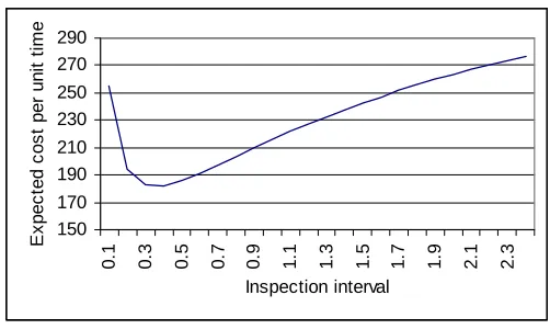
Assume both the initial time and delay time distributions are exponential with scale parameters 0.6 and 0.75 respectively. The time unit is 100 days and the cost parameter values are cf =£1000,cr = £150 and cs =£15 respectively. Using
150 170 190 210 230 250 270 290
0.
1
0.
3
0.
5
0.
7
0.
9
1.
1
1.
3
1.
5
1.
7
1.
9
2.
1
2.
3
Inspection interval
E
x
pec
ted
c
o
s
t per
uni
t t
im
[image:13.595.171.422.158.308.2]e
Fig 14.8 Expected cost per unit time v inspection interval
The optimal inspection interval is 0.4*100=40 days, so a monthly inspection schedule is appropriate.
14.4.2 Inspection model based on a non exponentially distributed initial time
If is not exponentially distributed, then we cannot assume any inspection will renew the system unless a defect was identified at an inspection and the system was replaced or repaired to as new condition. In this case a renewal cycle may span several inspection intervals.
)
(
u
g
Using a similar framework as before and now taking the expected downtime per renewal cycle as an example, the expected downtime due to a failure renewal at time
X
, whereX
∈
[(
i
−
1
)
T
,
iT
)
is∫
−−
+
−
=
<
<
−
+
−
iTT i f s f
s
d
P
i
X
iT
i
d
d
g
u
F
iT
u
du
d
i
) 1
(
(
)
(
)
]
)
1
[(
)
)
1
((
]
)
1
[(
(14.15)
This is because inspections are perfect so that if a failure at time X, then the initial time
U
must be bounded within[(
i
−
1
)
T
,
X
),
X
<
iT
. There are inspections with no defect identified before the failure so)
1
(
i
−
)
1
(
i
−
times of the inspection downtime are added.∑
∫
∑
∞ = − ∞ =−
+
−
=
<
<
−
+
−
1 ( 1)
1
)
(
)
(
]
)
1
[(
)
)
1
((
]
)
1
[(
i iT T i f si s f
du
u
iT
F
u
g
d
d
i
iT
X
i
P
d
d
i
(14.16)Equation 14.16 is always finite since all the probability terms for large
i
tend to zero becauseg
(
u
)
tends to zero foru
>
(
i
−
1
)
T
wheni
is large.Similarly the expected downtime due to an inspection renewal with a defect identified is
∑
∞∫
=1
((
−
1
)
+
)
(−1)(
)[
1
−
(
−
)]
i
iT
T i r
s
d
g
u
F
iT
u
du
d
i
(14.17)Summing (14.16) and (14.17) gives the complete expected downtime per renewal cycle
{
}
∑
∞∫
∫
=−
+
−+
−
−−
=
1 ) 1 ( ) 1 ((
)
(
)
(
)
(
)
]
)
1
[(
i iT T i r f iT T i rs
d
g
u
du
d
d
g
u
F
iT
u
du
d
i
E(CD)
(14.18)
The expected cycle length is obtained in a similar manner and is given by
{
}
∑
∞∫
∫
∫
= − −−
+
−−
−
=
1 ) 1 ( ) 1 ( ) 1(
(
)
(
)
(
){
1
(
)}
)
(
i iT T i t T i iT Ti
t
g
u
f
t
u
du
dt
iT
g
u
F
iT
u
du
CL
E
(14.19)
Finally the expected downtime per unit time is given by
{
}
{
}
∑
∫
∫
∫
∑
∫
∫
∞ = − − − ∞ = − −−
−
+
−
−
−
+
+
−
=
1 ( 1) ( 1) ( 1)
1 ( 1) ( 1)
}
)]
(
1
)[
(
)
(
)
(
)
(
)
(
)
(
)
(
]
)
1
[(
i iT T i t T i iT T i i iT T i iT T i r f r sdu
u
iT
F
u
g
iT
dt
du
u
t
f
u
g
t
du
u
iT
F
u
g
d
d
du
u
g
d
d
i
C(T)
(14.20)14.4.3 A case example
and repairs carried out using history cards for each individual item of departmental equipment. Information available included purchase date, date of preventive maintenance, failures and some description of the work carried out. There were no costs recorded, but some estimated cost values were provided by the hospital staff. Following a discussion with the chief technician, it seemed best to focus on the following items, to ensure a sample of similar machine types, under heavy and constant use, with a usefully long history of failures, and with reasonably well-defined modes of failures. Two pumps were chosen, namely volumetric infusion pumps and peristaltic pumps all from the intensive-care, neurosurgery and heart-care units. There were 105 volumetric pumps and the most frequent failure mode was the failure of the pressure transducer. There were 35 peristaltic pumps and the most frequent failure mode was battery failure. For a detailed description of the case, data and model fitting, see Baker and Wang (1991). Several distributions were chosen for the initial and delay time distributions for both pumps, and it turned out that in both cases a Weibull distribution was the best for the initial time distribution and an exponential distribution for the delay time distribution. The estimated parameter values based on history data using the maximum likelihood method for both pumps are shown in table 14.1.
Pump Initial time pdf.
η
α β
α
αη
(
)
1 ( ))
(
ue
u
u
g
=
− −Delay time pdf.
h
e
h
f
(
)
=
β
−βVolumetric infusion
α
ˆ
=0.0017,η
ˆ
=1.42β
ˆ
[image:15.595.124.472.377.466.2]=0.0174 Peristaltic
α
ˆ
=0.0007,η
ˆ
=2.41β
ˆ
=0.0093Table 14.1 Estimated parameter values for the pumps
Although the cost data were not recorded, it was relatively easy to estimate the cost of an inspection (called preventive maintenance in the hospital) and the cost of an inspection repair if a defect was identified. However, it was extremely difficult to have an estimate for the failure cost since if the pump failed to work while needed the penalty cost could be very high compared with the cost of the pump itself. Nevertheless, some estimates were provided, which are shown in table 14.2
Pump Inspection cost Inspection repair
cost Failure cost Volumetric infusion £15 £50 £2000
Peristaltic £15 £70 £1000
Table 14.2 Cost estimates
[image:15.595.125.474.574.636.2]calculate (14.20). We did this using the maths software package MathCad and the results are shown in Figs 14.9 and 14.10.
0 20 40 60 80 100 120
1.2 1.4 1.6 1.8 2 2.2 2.4
Expected_Cost T( )
T
[image:16.595.164.448.201.397.2]C(T)
Figure 14.9. Expected cost per unit time v inspection interval for the volumetric infusion pump
0 20 40 60 80 100 12
0.5 1 1.5 2 2.5
0 Expected_Cost T( )
T
C(T)
[image:16.595.169.454.452.653.2]Time is given in days in Figs 14.9 and 14.10, so the optimal inspection interval for the volumetric infusion pump is about 30 days and for the peristaltic pump is around 70 days. The hospital at the time checked the pumps at an interval of 6 months, so clearly for both pumps the inspection intervals should be shortened. However, it has to be pointed out that the model is sensitive to the failure cost, and had a different estimate been provided, the recommendation would have been different.
14.5 Delay Time Model Parameter Estimation
14.5.1 Introduction
In previous sections, delay time models for both a complex system and a single compnent have been introduced. However in a practical situation, before the construction of expected cost or downtime models, it is necessary to estimate the values of the parameters that characterise the defect arrival and failure processes. In this section we discuss various methods developed to estimate the parameters from either ‘subjective’ data of experts opinions or ‘objective’ data collected at failures and inspections.
Naturally, the parameter estimation process is not the same for the different types of delay-time model i.e. single component models where a single potential failure mode is modelled and only one defect may (or may not) be present at any one time, compared with complex system models where many defects can exist simultaneously and many failures can occur in the interval between inspections. This is particularly important for the method using objective data. In this section, we mainly focus on the estimation methods for complex systems since these systems are the most applicable asset items for DTM. The details of the approaches developed for parameters estimation for a single component DTM can be found in Baker and Wang (1991) and Baker and Wang (1993).
14.5.2 Subjective data method
Subjective estimation of the delay times through an on-site and on-spot survey This method needs to be done over a time period to collect detailed information and assessment at every maintenance intervention or failure, Christer and Waller (1984).
At every failure repair, the maintenance technician repairing the plant would be asked to estimate:
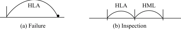
HLA: How long ago the defect causing the failure may first have been expected to have been recognised at an inspection.
If a defect was identified at an inspection, then in addition to HLA, the technician would be asked to estimate
HML: How much longer could the defect be left unattended before a repair was essential.
The estimates are given by, see Fig. 14.11 (a) and (b), for a failure, and for an inspection repair. is then estimated from the data
of { }.
HLA
h
ˆ
=
HML
HLA
h
ˆ
=
+
f
(
h
)
h
ˆ
HLA HLA HML ●
[image:18.595.164.466.375.426.2](a) Failure (b) Inspection
Figure 14.11 HLA and HML estimates at failure and inspection
At the time of repair, the maintenance technician has information available to inform his estimate. In addition to his experience, the defect is present, the plant may be examined, and operatives questioned.
The rate of defect arrivals can be estimated directly from the number of observed failures and defects identified over the survey period. For a case study using this approach for estimating delay time model parameters, see Christer and Waller (1984).
Subjective estimation of the delay times based idetified failure modes
Wang (1997) recommended a new approach to estimate directly the delay time distribution based on pre-defined major failure modes or types. The idea is as follows
1. If the estimates can be made based on pre-selected major failure types instead of the individual failure or defect when it occurs, the time spent for the questionnaire survey will be greatly reduced since the estimates for all major failure types can be carried out at the same time, which may only take a few hours. This also creates the opportunity for an analyst to be present to reduce possible confusion and mistakes.
2. A group of experts should be questioned on the same failure type and opinions can be properly combined to reduce sampling errors.
3. The question asked should be a probabilistic measure of the delay time over all possible ranges.
The following phases for the estimating of the delay time were suggested, Wang (1997).
The problem identification phase
This is for the identification of all major failure types and possible causes of the failures. This was normally done via a failure mode and criticality analysis so that a list of dominant failures can be obtained. This process will entail a series of discussions with the maintenance engineers to clarify any hidden issues. If some failure data exists it should be used to validate the list, or otherwise a questionnaire should be designed and forwarded to the person concerned for a list of dominant failure types.
Expert identification and choice phase
The term ‘expert’ is not defined by any quantitative measure of resident knowledge. However, it is clear in the case here that a person who is regarded by others as being one of the most knowledgeable about the machine should be chosen as the expert. The shop floor fitters or any maintenance technicians or engineers who maintain the machine would be the desired experts, Christer and Waller (1984). After the set of experts is identified, a choice is made which experts to use in the study. Full discussion with management is necessary in order to select the persons who know the machine ‘best’. Psychologically, five or fewer experts are expected to take part of the exercise, but not less than three.
The question formulation phase
The questions we want to ask in this case are the rate of occurrence of defects, (assuming we are modelling a complex plant) and the delay time distribution. In the case addressing the rate of arrival of a defect type, we can simply ask for a point estimate since it is not random variable. Without maintenance interventions, this would, in the long term, be equal to the average number of the same failure type per unit time. For example we may ask ‘how many failures of this type will occur per year, month, week or day?’. It is noted that this quantity is usually observable. In fact, our focus is mainly on the delay time estimates.
to communicate something about the range of their uncertainty. Accepting these points, perhaps the best that experts could do in this case would be to give their subjective probability mass function for the quantity in question. In other words, they could provide an estimate over the interval such that the mass above the interval is proportional to their subjective probability measures. Alternatively, three point estimates can be asked, such as the most likely, the minimum and the maximum durations of the delay times for a particular type of failure.
The word ‘delay time’ was not entered in the question since it will take some effort to explain what is the delay time. Instead, we just asked a similar question like HLA. But this question was still difficult for the experts to understand based upon our case experience. The lesson learned is to demonstrate one example for them before starting the session.
The elicitation phase
Elicitation should be performed with each expert individually. If possible, the analyst should be present, which proved to be vital in our case studies. The above mentioned histogram was used to draw the answer from the experts so that the experts can have a visual overview of their estimates and a smooth histogram could be achieved if the experts are advised to do so. The maximum number of the histogram intervals is set to be five, which is advised by psychological experiments.
The calibration phase
Roughly speaking, calibration is intended to measure the extent to which a set of probability mass functions ‘correspond to reality’. Reviewing the problem we have concluded that subjective calibration is not recommended due to its time consuming nature. If any objective data is available, we may calibrate the experts’ opinion by a Bayesian approach as discussed by many others. Other approach is to calibrate the estimate by matching a statistics observed. If significant difference is found, the estimates must be revised.
The combination phase
Experts resolution, or combining probabilities from experts, has received some attention. Here we use one of the simplest approaches, namely the weighting method. It is simply a weighted average of the estimates of all experts. The weights need to be selected carefully according to each expert’s level of expertise, and their sum should be equal to one. Other more complicated methods are available, see Wang (1997)
It is noted that the combined delay time distribution obtained from this phase is in a form of discrete probability distribution. In fact a continuous delay time distribution is needed in delay time inspection modelling. To achieve this, based upon the number of delay times in each interval, an estimated continuous delay time distribution of can be obtained by fitting a distribution from a known family failure distributions, such as exponential or Weibull using the least square method or maximum likelihood method.
)
(
ˆ
h
The updating phase
This phase is mainly for after some failure and recorded findings become available. In a sense it is a way of calibrating.
A case study using the above method is detailed in Akbarov et al (2006).
An empirical Bayesian approach for estimating the DTM parameters based subjective data
In previous subjective data based delay time estimating approaches, Christer and Waller (1984), Wang (1997), and Akbarov et al (2006), some direct subjective estimates of the delay time is required, which has been found to be extremely difficult for the experts to estimate since the delay time is not usually observable and difficult to explain, Akbarov et al (2006).
We now introduce a recently developed new approach which starts with subjective data first and then updates the estimates when objective data becomes available. The initial estimates are made using the empirical Bayesian method matching with a few subjective summary statistics provided by the experts. These statistics should be designed easy to get based on the experience of the experts and on observed practice rather than unobservable delay times. Then the updating mechanism enters the process when objective data become available, which requires a repeated evaluation of the likelihood function which will be introduced later. In the framework of Bayesian statistics and assuming no objective data is available at the beginning, we basically first assume a prior on the parameters which characterize the underlying defect and failure arrival processes. When objective data becomes available, we calculate the joint posterior distribution of the parameters, and then we may use this posterior distribution to evaluate the expected cost or downtime per unit time conditional on observed data.
Assuming for now that we are interested in the rate of arrival of defects,
λ
, and the delay time pdf.,f
(
h
)
, which is characterised by a two parameter distribution)
,
|
(
h
α
β
f
. Unlike the methods proposed in Christer and Waller (1984), Wang (1997), here we treat parametersλ
and theα
andβ
inf
(
h
|
α
,
β
)
as random variables. The classical Bayesian approach is used here to define the prior distributions for model parametersλ
,α
andβ
asf
(
λ
|
Φ
λ)
,)
|
(
α
Φ
αf
andf
(
β
|
Φ
β)
, whereΦ
•is the set of hyper-parameters within .)
|
(
•
Φ
•f
Once those
Φ
• are available, the point estimates ofλ
,α
andβ
are the expected values of them and are given by∫
∫
∫
∞ Φ = ∞ = ∞ Φ=
0 0
0 ( | )
ˆ and ) ( ˆ
, ) | (
ˆ
λ
λ
λ
α
α
α
α
β
β
β
β
λ
f λ d f |Φα d f β d)] , , (
[g Φλ Φα Φβ
E denote its expected value in terms of
Φ
λ,Φ
α and ,then we have
β
Φ
.
)
|
(
)
|
(
)
|
(
)
,
,
(
)]
,
,
(
[
0 0 0
∫ ∫ ∫
∞ ∞ ∞Φ
Φ
Φ
=
Φ
Φ
Φ
β
α
λ
β
α
λ
β
α
λ
λ α ββ α λ
d
d
d
f
f
f
g
g
E
(14.21)If we can obtain a subjective estimate of E[g(Φλ,Φα,Φβ)] provided by the experts, denoted by
g
s, then letting E[g(Φλ,Φα,Φβ)]=gs, we have∫ ∫ ∫
∞ ∞ ∞Φ
Φ
Φ
=
0 0 0
g
(
λ
,
α
,
β
)
f
(
λ
|
λ)
f
(
α
|
α)
f
(
β
|
β)
d
λ
d
α
d
β
.
g
s (14.22)Equation 14.22 is only one of such equations and if several such subjective estimates (different) were provided, we could have a set of equations 14.22. The hyper-parameters may be estimated by solving equations 14.22 in the case that the number of equations 14.22 is at least the same as the number of hyper-parameters in . We now demonstrate this in our case.
•
Φ
•
Φ
Suppose that the experts can provide us the following subjective statistics in estimating
Φ
λ:• The average number of failures within
[
0
,
T
)
, denoted by ,n
f• The average number of defects identified at inspection time
T
, denoted byd
n
• The average probability of no defect at all in
[
0
,
T
)
, denoted byp
nd.In this case if the statistics of interest is the average number of the defects within , we have from the property of the HPP that
)
,
0
[
T
g
(
λ
,
α
,
β
)
=
λ
T
, and then∫
∫ ∫ ∫
∞ ∞ ∞ Φ Φ Φ = ∞ Φ=
Φ Φ Φ
0
0 0 0 ( | ) ( | ) ( | ) ( | )
)] , , ( [
λ
λ
λ
β
α
λ
β
α
λ
λ
λ α β λβ α λ d Tf d d d f f Tf g E
Since if inspection is perfect we have
g
s=
n
f+
n
d, it follows from (14 .22) that.
)
|
(
0
λ
Tf
λ
λd
λ
n
Similarly, from the property of the HPP, that is, ! ) ( e ) | n T) (0, ( T -n T N P n d λ λ = λ
= , we have . ) | ( ) | ( ) | 0 T) (0, ( 0
0
λ
λ
λ
λ
λλ
λ
λ d e f d
f N
P
pnd
∫
r d∫
T∞ − ∞ Φ = Φ =
= (14.24)
where is the number of defects in . If we have only two hyper-parameters in , then solving (14.23) and (14.24) simultaneously in terms of
will give the estimated values of the hyper-parameters in
)
,
0
(
T
N
d[
0
,
T
)
λ
Φ
λ
Φ
Φ
λ. Note thatλ
is independent with
α
andβ
so that the integrals of f(α|Φα)and f(β
|Φβ)are dropped from (14.21). Similarly if more subjective estimates were provided, the hyper-parameters in
Φ
α andΦ
βcan be obtained. For a detailed description of such an approach to estimate delay time model parameters see Wang and Jia (2007).Obviously this approach is better than the previously developed subjective methods in terms of the way to get the data and the accuracy of the estimated parameters. It is also naturally linked to the objective method in estimation DTM parameters to be presented in the next section via Bayesian theorem if such objective data becomes available, Wang and Jia (2007).
14.5.3 Objective data method
Objective data for complex systems under regular inspections should consist of the failures (and associated times) in each interval of operation between inspections and the number of defects found in the system at each inspection. From this data information, we estimate the parameters for the chosen form of the delay time model.
Initially, we consider a simple case of the estimation problem for the basic delay time model where only the number of failures, , occurring in each cycle
and the number of defects found and repaired, , at each inspection (at time
iT
) are required. We do not know the actual failure times within the cycles im
)
),
1
[(
i
−
iT
j
iThe probability of observing
m
i failures in[(
i
−
1
),
iT
)
is;(
)
! )] , ) 1 (( [ ) , ) 1 (( )] , ) 1 (( [ i m f iT T i N E i f m iT T i N E e m iT T i N P i f − = = − − − (14.25)(
)
!
)]
(
[
)
(
)] ( [ i j s iT N E i sj
iT
N
E
e
j
iT
N
P
i s −=
=
(14.26)As the observations are independent, the likelihood of observing the given data set is just the product of the Poisson probabilities of observing each cycle of data, and
i
m
i
j
. As such, the likelihood function forK
intervals of data is;∏
= − − − ⎪⎭ ⎪ ⎬ ⎫ ⎪⎩ ⎪ ⎨ ⎧ ⎟ ⎟ ⎠ ⎞ ⎜ ⎜ ⎝ ⎛ ⎟ ⎟ ⎠ ⎞ ⎜ ⎜ ⎝ ⎛ − = Θ K i i j s iT N E i m f iT T i N E j iT N E e m iT T i N E e L i s i f 1 )] ( [ )] , ) 1 (( [ ! )] ( [ ! )] , ) 1 (( [ ) ( , (14.27)where is the set of parameters within the delay time model. The likelihood function is optimised with respect to the parameters to obtain the estimated values. This process can be simplified by taking natural logarithms. The log-likelihood function is;
Θ
(
)
(
)
∑
∑
= = + − − − − + − = Θ Ki i i
K
i i f i s f s
j m iT N E iT T i N E iT N E j iT T i N E m 1 1 ) ! log( ) ! log( )] ( [ )] , ) 1 (( [ )]} ( [ log{ )]} , ) 1 (( [ log{ ) ( A (14.28)
where the final summation term is irrelevant when maximising the log-likelihood as it is a constant term and therefore not a function of any of the parameters under investigation.
When the times of failures are available, it is often necessary to refine the likelihood function, (14.27) by considering the detailed pattern of behaviour within each interval in terms of the number of failures and their associated times. Define the time of the jth failure in the ith inspection interval, the likelihood is given by, Christer et al (1998),
ij
t
∏ ∏
= − − − = ⎪⎭ ⎪ ⎬ ⎫ ⎪⎩ ⎪ ⎨ ⎧ ⎟ ⎟ ⎠ ⎞ ⎜ ⎜ ⎝ ⎛ = Θ K i i j s iT N E iT T i N E mj i ij j
iT N E e e t v L i s f i 1 )] ( [ )] , ) 1 (( [ 1 ! )] ( [ ) ( ) ( (14.29)
where
v
i(
t
ij)
is given by (14.4).data. It was done essentially by formulating the probability of a particular number of failures for each day over each inspection interval, and then the likelihood for a particular inspection interval is just the product of these probabilities and the probabilty of observing some number of defects at the inspection, see Chriter et al (1995) for details.
14.5.4 A case example
A copper works at the Northwest England was used for same extrusion press for over 30 years, and the plant is a key item in the works since 70% of its products shall go through this press at some stage of their production. The machine comprises a 1700-ton oil-hydraulic extrusion press with one 1700kW induction heater and completely mechanized gear for the supply of billets to the press and for the removal of the extruded products. The machine was operated 15-18 hours a day (two shits), 5 days a week, excluding holidays and maintenance down-time. Preventive Maintenance (PM) was carried out on this machine since 1993, which consisted of a thorough inspection of the machinery, along with any subsequent adjustments or repairs if the defects found can be rectified within the PM period. Any major defects which cannot be rectified during the PM time were supposed to be dealt with during non-production hours. PM lasted about two hours and is performed once a week at the beginning of each week.
Questions of concern are (i) whether PM is or could be effective for this machine; (ii) whether the current PM period is the right choice, particularly, the one week PM interval which was based upon maintenance engineers’ subjective judgement; (iii) whether PM is efficient, i.e. whether it can identify most defects present and reduce the number of failures caused by those defects.
In this case study, the delay time model introduced earlier was used to address the above questions. The first question can also be answered in part by comparing the total downtime per week under PM with the total downtime per week per week of the previous years without PM. A parallel study carried out by the company revealed that PM has lowered the total downtime. The proportion of downtime was reduced from 7.8% to 5.8%.
To establish the relationship between the downtime measure and the PM activities using the delay time concept, the first task is to estimate the parameters of the underlying delay time distribution from available data, and hence build a model to describe the failure and PM processes. The type of delay time model used in the study is the non-perfect inspection model.
In the original study, Christer et al (1995), a number of different candidate delay time distributions were considered including exponential and Weibull distributions. The chosen form for the delay time distribution is a mixed distribution consisting of an exponential distribution (scale parameter α) with a proportion P of defects having a delay time of 0. The cdf. is given by
h
-P
-(
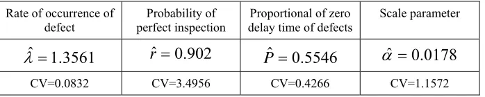
An optimisation algorithm is required for maximisation of the likelihood with respect to the parameters. The estimated values are given in table 14.3 with their associated coefficients of variation (CV)
Rate of occurrence of
defect perfect inspection Probability of delay time of defects Proportional of zero Scale parameter
3561
.
1
ˆ
=
λ
r
ˆ
=
0
.
902
P
ˆ
=
0
.
5546
α
ˆ
=
0
.
0178
[image:26.595.126.475.204.274.2]CV=0.0832 CV=3.4956 CV=0.4266 CV=1.1572
Table 14.3 Estimated model parameters
Inserting the optimal parameter estimates into the log-likelihood function gives a ML value of 101.86. See Christer et al (1995) on the analysis and the fit of the model to the data.
14.6 Other developments in DTM and future research
Several useful extensions have been made over the last decade to make the delay time model more realistic, but that increases the mathematical complexity as well. Christer and Wang (1995) addressed an NHPP non-perfect inspection delay time model of multiple component systems. In this case the constant inspection interval assumption cannot be held, and a recursive algorithm was developed in Wang and Christer (2003) to find the optimal non-constant intervals till final replacement. Christer and Redmond (1990) reported a problem of sampling bias, and proposed ways of estimating the delay time distribution from subjective data. Wang and Christer (1997) modelled a single component system subject to inspections over a finite time horizon. Christer et al (1997) used a NHPP in modelling the rate of arrival of defects within a case study. Wang (2000) developed a model of nested inspections using the delay time concept. Wang and Jia (2006) reported the use of empirical Bayesian statistics in the estimation of delay time model parameters using subjective data, which overcame a number of problems in previous subjective delay time parameter estimation. If the downtime due to failures cannot be ignored in the calculation of the expected number of failures during an inspection interval, Christer et al (2000) addressed this problem and a refined method was proposed. Christer et al (2001) compared the delay time model with an equivalent semi-Markov setting to explore the robustness of both modelling techniques to the Markov assumption. Carr and Christer (2003) in a recent paper, studied the problems of non-perfect repairs at failures, which allows failures to re-occur if the repair is not perfect.
The future research on the DTM relies on the application areas, the data involved, and the objective function chosen. We consider that the following areas or problems are worthy of research using the delay time concept.