A constraint manager to support virtual
maintainability
Marcelino, L, Fernando, T and Murray, N
http://dx.doi.org/10.1016/S00978493(02)002285
Title
A constraint manager to support virtual maintainability
Authors
Marcelino, L, Fernando, T and Murray, N
Type
Article
URL
This version is available at: http://usir.salford.ac.uk/917/
Published Date
2003
USIR is a digital collection of the research output of the University of Salford. Where copyright
permits, full text material held in the repository is made freely available online and can be read,
downloaded and copied for noncommercial private study or research purposes. Please check the
manuscript for any further copyright restrictions.
A Constraint Manager
to Support Virtual Maintainability
Luis Marcelino
Norman Murray
Terrence Fernando
Centre for Virtual Environments, University of Salford Salford, U.K.
{L.Marcelino,T.Fernando,[email protected]
Abstract
Virtual prototyping tools have already captivated the industry's interest as a viable design tool. One of the key challenges for the research community is to extend the capabilities of Virtual Reality technology beyond its current scope of ergonomics and design reviews. The research presented in this paper is part of a larger re-search programme that aims to perform maintainability assessment on virtual prototypes. This paper discusses the design and implementation of a geometric constraint manager that has been designed to support physical realism and interactive assembly and disassembly tasks within virtual environments. The key techniques em-ployed by the constraint manager are direct interaction, automatic constraint recognition, constraint satisfac-tion and constrained mosatisfac-tion. Various optimisasatisfac-tion techniques have been implemented to achieve real-time in-teraction with large industrial models.
Keywords
1. INTRODUCTION
Modern markets not only urge companies to create better products, but also force them to do so in increasingly shorter time scales. The concept of Concurrent Engi-neering (CE) encourages companies to address issues such as maintenance very early in the design process. However, the lack of simulation tools hinders the adapta-tion of CE and therefore further research is required to develop such tools. A development stage that is still lacking the appropriate software tools is maintenance simulation. The simulation of maintenance operations allows maintenance to be addressed in early design stages. This reduces unforeseen problems creeping into the design as it progresses through its life cycle, conse-quently saving both time and money while improving product quality.
The Virtual Prototyping Group at the Centre for Virtual Environments at Salford has been investigating the ap-plicability of VR to interactive maintenance simulation. A system that can simulate realistic maintenance opera-tions interactively is demanded by the industry. This research inverstigates the use of virtual environments to assess maintenance operations before any physical proto-type is available. Besides speeding up the development process, the assessment of virtual models can also reduce the number of required physical prototypes. Such a tool has the potential to reduce the time-to-market and the development cost.
Maintenance operations are usually performed in a re-stricted space within a limited timespan. The operator's movements are often constrained by the surrounding components and contacts and clashes between compo-nents are inevitable. Furthermore, the time required for maintenance needs to be controlled and minimized. For these issues to be considered in a maintenance simula-tion, the computer simulation needs to be realistic.
To achieve a real-time realistic simulation we use a geo-metric constraint approach. Geogeo-metric constraints are relationships established between different geometric primitives. These relationships constrain the movement of objects and determine the objects' kinematics. The use of geometric constraints has two advantages against the alternative physical simulation: it is less computationally intensive, and only requires the information already available in CAD models. The more accurate physical simulation needs extra information like mass, friction coefficient, etc.
assem-assembly and disassem-assembly operations in immersive vir-tual environments.
The next section introduces some of the work done in virtual maintainability. Section 3 describes some of this system's functionality and Section 4 presents its architec-ture and implementation. The simulation of maintenance tasks using a real industrial model required the con-straint manager to be optimised as described in Section 5. The CM performance using the industrial case study is presented in Section 6. Section 7 discusses the achieved results and defines the orientation for future work.
2. RELATED WORK
There have been several research efforts to develop as-sembly simulator environments and much work has been done allowing users to compose scenes within virtual environments, such as 3DM [Butterworth-92], and JDCAD [Liang-94] which tackled many of the issues involved in the interactive creation of 3D objects. Prob-lems with such systems are the absence of constraints when interacting with virtual objects. Users are restricted to gross interactions and are unable to perform precise object manipulation [Mine97]. Systems that support con-straint based assembly of components provide the user with the support required to position components pre-cisely in 3D space. There have been several research efforts to investigate the development of assembly simu-lation environments. For example, Connachar et al. [Connacher96] [Jayaram99] describes a system called VADE (Virtual Assembly Design Environment) inter-faced with the Pro/Engineer modelling environment. A CAD database is connected to the Open Inventor API through Pro/Engineer Pro Develop Toolkit. In this sys-tem, direct interaction is supported through a Cyber-Glove. Fernando et al. [Fernando95], Fa et al. [Fa93], Munlin [Munlin95], and Thomson et al. [Thompson98], have developed an Interactive Constraint Based Assem-bly Modelling (ICBAM) environment to bring physical realism to the assembly simulation arena. Zachmann [Zach01] developed an assembly simulator that imple-ment some constrained motion based on the type of con-tact between objects.
Fernando et al. [Fernando95] describes the methods de-veloped for allowable motion and constraint recognition within the system. Automatic recognition of constraints such as 'against', 'coincident', 'tangential', and 'concen-tric' are supported in their system. By reading constraint relationships stored in a Relationship Graph, degrees of freedom can be computed so that the system can deter-mine the allowable motions for a given assembly part. The VR environment is implemented using the IRIS Inventor graphical toolkit. The system described by Fer-nando et al. [FerFer-nando95] reported some shortcomings. They include, inability to support constraint propagation from child object to parent when the child object is being manipulated in the assembly, and the absence of a
stan-dard data translator for CAD data import into the virtual environment.
3. SYSTEM DEFINITION
This section presents the functionality of the constraint manager that was derived from its requirements. These requirements are based on previous experience building an assembly simulator [Wimalaratne01].
The development of a new constraint manager aimed to create an efficient and independent software toolkit that could be easily integrated into different virtual reality systems. The requirements for this system were:
• Multi-platform (UNIX and windows)
• Scene graph independence
• Multiple constraint recognition
• Multiple constraint satisfaction
• Deletion of broken constraints
• Automatic constraint management
The communication between the constraint manager and the main application uses a defined API with appropriate data structures. The internal data representation is based on private classes that are independent of any scene graph. For this reason the VR system needs to insert into the constraint manager each component's geometry, be-cause the constraint manager has its own internal data representation. This allows the main application to choose the objects that can be constrained. The virtual hand, for example, would not be inserted into the con-straint manager and therefore not be subject to geometric constraints.
The constraint manager has two types of geometry nodes: objects and surfaces. An object is an entity that has surfaces and can be moved. A surface is a face of an object. The constraint manager supports parametric sur-faces and uses specific elements that define its paramet-ric equation. For example a point on the plane and its normal vector defines a planar surface while a point on the cylinder axis, its direction and the radius of the cyl-inder value define a cylindrical surface. Besides surface specific elements, each surface has a bounding volume. This volume defines surface's borders because the equa-tions define limitless surfaces. The constraint manager has no polygonal representation of surfaces because such a representation is not relevant to the constraint man-agement process.
sup-ports the three different types of constraints illustrated in Figure 1.
[image:4.595.299.511.122.335.2](a) Against (b) Collinear (c) Concentric
Figure 1: Supported constraints
The constraint recognizer must also be able to validate recognized and applied constraints. The validation is the process that determines whether a constraint is still valid or is broken. A constraint is broken if the involved sur-faces attempt to move apart beyond a defined threshold.
The preferred way for the VR system to exchange data with the Constraint Manager is through the use of lists. The VR system can send to the constraint manager a list of surfaces with constraints to be added and the con-straint manager can return a list of surfaces with the recognized constraints. Lists are a convenient communi-cation medium because they do not restrict the amount of data passed to and from the constraint manager and a list received from the constraint manager can be freely manipulated by the application and then sent back to the constraint manager.
The functionality of the constraint manager can be di-vided in three main tasks:
• To validate existing constraints and determine the broken constraints;
• To enforce existing constraints and solve con-strained motion;
• To recognize new possible constraints.
This functionality can be combined to achieve three stage fully automated constraint manager. Once a com-ponent's transformation is passed to the constraint man-ager, the model is searched for possible broken con-straints that are removed. The remaining concon-straints are enforced and a resulting transformation computed. Once in a position, the constraints manager searched for new constraints between the moved component and the sur-rounding.
4. SYSTEM ARCHITECTURE
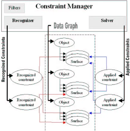
This section describes the architecture of the imple-mented constraint manager. Figure 2 shows a graphical representation of this architecture.
The constraint manager has a hierarchical data graph that maintains all relevant information from objects and surfaces. The data graph is available to all modules of
the constraint manager: the constraint solver, the con-straint recogniser and the filters. The concon-straint manager modules are independent and their interaction is defined by the application.
Figure 2: The Constraint Manager Architecture
4.1 The data-graph
The data graph is a hierarchical data structure that maintains the information relevant to the constraint manager. It represents all the knowledge the constraint manager has about the components within the virtual environment. This means the constraint engine has its own insight of the virtual environment. Virtual objects and surfaces that are not to be constrained are simply not added to the constraint engine and so are not considered during the solving and recognition process.
The data graph is organized like a flat scene-graph with the top-level nodes representing objects and the leaf-nodes representing surfaces. All objects and surfaces added to the constraint manager are in the data graph. A data graph's object is a node that has a list of surfaces and can be transformed. Valid transformations are lation and rotation, but not scale. An object can be trans-formed through direct manipulation or as a result of other object's movement. An object can be fixed in the 3D space to prevent it from being moved.
4.2 The constraint solver
The constraint solver maintains a list of the applied con-straints. Applied constraints are the constraints to be enforced and that condition objects' transformations. Constraints apply to surfaces of distinct objects only, because this library only supports rigid bodies. This means that different surfaces of the same object are al-ways fixed relative to each other and no constraint can be applied between them.
All transformations pass by the constraint solver. A new transformation for an object means that this object is being moved from its current position to a new one. The solver determines whether this motion is possible or not and, if not, it computes an alternative position. An ob-ject's motion can also affect the position of other con-strained objects. The solver also computes the new posi-tion of constrained objects and updates these objects po-sition.
4.3 The constraint recognizer
The constraint recognizer identifies new possible con-straints and validates existing ones. The application specifies a list of objects to be searched for new con-straints and possibly the surfaces to be tested for new constraints. If the application can determine collisions between surfaces, it can send those colliding surfaces to the constraint recognizer. This speeds up the recognition process because it cuts the number of surfaces to be tested.
The constraint recognizer has two lists of recognized constraints. Figure 2 shows only one of these lists for clarity. One list has the new recognized surfaces while the other has the existing constraints that failed to be recognized. These list of constraints are returned to the application, which then decides what to do with them. It is under the application's control to apply all, some or none of the recognized constraints, as it can control which constraints to break: all of those recognized, some of them or none of them.
The methods used for recognition of new constraints are also used to validate existing constraints. The validation process is based on the principle that a recognizable con-straint is still a valid one. Validation takes place before existing constraints are enforced, otherwise existing con-straints would always be recognized. Existing concon-straints that fail to be recognized are added to the list of broken constraint.
The constraint manager has a set of variables that define the tolerance of the recognition process. These tolerances determine the threshold under which constraints are rec-ognized and can be adjusted dynamically by the applica-tion. The three recognition tolerances are the linear tol-erance, the angular tolerance and the breaking factor. The linear tolerance is the maximum distance between two surfaces (or axis if two cylinders are involved), the angular tolerance is the maximum angle between two surfaces and the breaking factor is the scaling factor that multiplies the linear and angular tolerances when
con-straints are being validated. A breaking factor greater than 1 means it is easier to recognize new constraints than to break existing ones. Increasing the breaking fac-tor makes constraints more difficult to break.
The constraint recognition algorithm compares surfaces and verifies if their relative positions and orientations are within the specified tolerances. The application de-fines a list of surfaces that the recognizer uses to search possible constraints. Alternatively objects can be inserted into this list, in which case the recognizer searches all surfaces of those objects for possible constraints. The recognition process starts with a bounding box intersec-tion test. To include the tolerance in the bounding box test, both surface boxes are enlarged by half the tolerance values. If bounding boxes are overlapping, the surfaces relative position and orientation is assessed to recognise possible constraints.
A constraint is recognized between two planes when the angle between their normals is less than the angular tol-erance and that the distance between the planes is less than the linear tolerance. Two cylinders have a potential constraint when their axes make an angle within the angular tolerance and are less than the tolerance apart. The constraint between a plane and a cylinder is recog-nized if a plane's normal it perpendicular within the tol-erance to the cylinder's axis and if the distance between the cylindrical and the planar surface is less than the linear tolerance.
4.4 Filters
Filtering is required to reduce the number of recognized constraints to a minimum. It takes three constraints to completely fix an object to other. Filters are functions that selectively remove recognized constraints from their list. The need for a filtering mechanism was raised when we tested the constraint manager with industrial case studies. These models do not have optimised surfaces and what could be one surface is sometimes a collection of small surfaces of the same type. As a result, recogni-tion of geometric constraints often generates a large number of possible but redundant constraints. Filters reduce the constraint list according to their criteria and are mutually independent. The application chooses what filters to apply to the list of recognized constraints and in which order.
Some of the filters currently provided by the constraint manager include:
• Surface displacement: filters the constraint of a specified type that have closer surfaces;
• Cylinder radius: remove concentric constraints detected between cylinders of different radii;
• Cylinder definition: removes duplicated cylin-drical constraints involving different cylincylin-drical surfaces with identical geometry;
5. SYSTEM OPTIMISATION
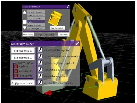
The use of the constraint manager with real industrial case studies revealed that the constraint manager did not scale up to support real industrial models. The models used by the industry are significantly more complex than
[image:6.595.66.516.116.455.2]the models used during the implementation of the con-straint manager. The test model shown in Figure 3 in-volved assembling components with approximately 20 surfaces each while the industrial case study involved one
Figure 3: An interface to the Constraint Manager with the original model
component with more than 800 surfaces and others with more than 50.
An assessment using the industrial case study revealed two bottlenecks in the constraint manager. One was the recognition process and the other was the transformation of objects. Using the industrial model the constraint manager needed nearly 200 milliseconds to recognize constraints and 80 milliseconds to move constrained objects. Surprisingly the constraint solver also needed approximately 70 milliseconds to move unconstrained objects. These two bottlenecks resulted in unacceptably low frame rate.
Several techniques were implemented to improve the performance of the constraint manager. This paper only presents the adopted solutions that are now part of the constraint manager.
5.1 The recognizer optimisation
The constraint recognizer was integrated in a VR frame-work that was adding pairs of objects, instead of pairs of surfaces, into the list to be recognized. The recognizer
ognizer then created a list of surface pairs from all pos-sible surfaces combinations. One object with X surfaces and another with Y surfaces resulted in X*Y surface pairs. Recognizing constraints between two components from the original model required 400 surface pairs to be tested while with the industrial case study this number increased to 40000 surface pairs.
The spatial filtering is a pre-processing step that is done when a component is added to the constraint manager. A bounding box is created for each component by adding the bounding boxes of all its surfaces. The component's bounding box is then divided into eight equal spatial cells and each surface is assigned to the spatial cells it uses.
Prior to recognising constraints between surfaces of two components the recognizer determines which cells of each component are intersecting. This information is then used to filter the surfaces pairs to be tested: only surfaces that are in intersecting cells are searched for possible constraints.
The association of spatial information to surfaces re-duced considerably the number of surfaces to be consid-ered in the recognition of new constraints. Using this new implementation the recognizer does in less than 30 milliseconds what previously took nearly 200 millisec-onds for the chosen industrial case study.
5.2 The solver optimisation
All components are transformed using the constraint manager. The constraint manager receives a requested transformation and passes it to the solver. The solver determines the final transformation of objects enforcing applied constraints. The performance assessment showed that the 3D DCM library was using most of the time, even for unconstrained objects. The experiments also revealed that the time required to transform components depended more on the complexity of the components than on the applied constraints.
From the obtained results it was clear that to improve the solver performance we needed to reduce the number of surfaces inserted into the 3D DCM. All components added to the constraint manager are inserted into the DCM as bodies without surfaces. The data graph still maintains both objects and surfaces data and only infor-mation inserted into the 3D DCM library is simplified. Surfaces are only inserted into the DCM as required, i.e. when they are constrained. This way the DCM library is abstracted from the complexity of components and only deals with very simple bodies. As a result the perform-ance of the constraint solver now depends on the number of applied constraints.
6. EXPERIMENTAL RESULTS
This section presents the performance results of the con-straints manager using a real industrial case study. The three main processing stages are assessed.
[image:7.595.300.528.55.275.2]The computer used to this experiments was an SGI ONYX2 with 128MB of RAM and two MIPS R10000 CPUs clocked at 180Mhz. However, the constraint man-ager is single threaded and only one CPU was used at a time.
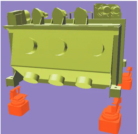
Figure 4: The Sener electronic box and its brackets
The model used in this experiment is a real case study from Sener, one of our industrial partners. The model has one electronic box and four brackets where it clamps. Some pipes and tubes are also part of the model but were not constrained. The electronic box is a compo-nent that has 872 surfaces and each bracket has 275 sur-faces. This experiment consisted of the manipulation of the electronic box so it automatically recognizes con-straints with one of the brackets. Once the electronic box clamps into the bracket it then moves along with the electronic box because it is not fixed within the world.
Figure 5: Automatic constraints recognition of two components with 872 and 275 surfaces.
[image:7.595.300.526.437.630.2]Figure 6: Time required transforming a component.
The time required to move objects was also reduced sig-nificantly due to the solver optimisation discussed in section 5.2. Figure 6 shows how the time to move the electronic box relates with the applied constraints. The "static surface" shows the time when all surfaces are inserted into 3D DCM while the "dynamic surface" when only constrained surfaces are inserted into the 3D DCM. Besides showing the performance improvement achieved by dynamically adding surfaces Figure 6 also shows the time 3D DCM needs when constraints are applied. This jump is due to the resetting of 3D DCM and happens every time constraints or geometries are added into, or removed from the library.
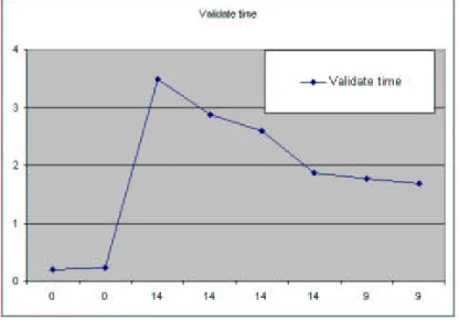
Figure 7: Time to validate existing constraints.
The validation time was inferior to the other two proc-essing stages. Figure 7 shows that less than four milli-seconds are needed to positively validate 14 existing constraints.
7. CONCLUSIONS AND FUTURE WORK
The results presented in the previous section demon-strate that the constraint manager can be used in interac-tive maintenance simulation of industrial models. The initial implementation of the constraint manager re-quired approximately 250 milliseconds per interaction for fully automated constraint management and as a re-sult could not be used interactively. The optimised
ver-sion of the constraint manager needs approximately 50 milliseconds to do the same job. We find this is an ac-ceptable simulation time given the complexity of the used components.
Despite the good results there is plenty of work to be done to achieve a mature system that can be used as a virtual prototyping tool. Further improvements to the existing constraint manager are now being considered. These improvements consist of developing a more effi-cient spatial data structure and applying filters before the recognition of new constraints.
8. ACKNOWLEDGEMENTS
This work has been supported by the EPSRC through a joint project with Rolls-Royce, EDS Parasolid and D-Cubed.
We would like to thank to Sener for providing the case study used in these experiments.
9. REFERENCES
[Butterworth-92] Butterworth, J., Davidson, A., Hench, S., Olano, T., “3DM: A Three-Dimensional Modeler Using a Head-Mounted Display”, ACM Computer Graphics (1992 Symposium on Interactive 3D Graphics), Volume 25 (2), 1992, pp. 135—138
[Connacher96] Connacher, H. and Jayaram, S. and Ly-nos, K., “Integration of Virtual Assembly with CAD”, Symposium on Virtual Reality in Manufacturing Research and Education, October 1996, pp. 32—40
[Cruz-Neira-93] Cruz-Neira, C., Sandin, D., DeFanti, T., "Surround-Screen Projection-Based Virtual Real-ity: The Design and Implementation of the CAVE", Proceedings of the 20th annual conference on Com-puter graphics, Anaheim, USA, 1993, pp. 135—142
[image:8.595.53.261.419.564.2][Cutler97] Cutler, L and Froehlich, B. and Hanrahan, P., "Two-Handed Direct Manipulation on the Respon-sive Workbench", Proceedings of the 1997 Sympo-sium on Interactive 3D Graphics, Providence, USA, April 1997
[dcubed01] Cubed, Ltd, “The 3D DCM Manual”, D-Cubed, Ltd, Version 2.5.0, August 2001
[Fa93] Fa, M., “Interactive Constraint-Based Assembly Modelling”, Ph.D. Thesis, School of Computer Stud-ies, University of Leeds, Sept, 1993
[Fernando00] Fernando, T, Marcelino, L, Wimalaratne, P, Tan, K, “Interactive Assembly Modelling within a CAVE Environment”, 9 Eurographics Portuguese Chapter Meeting, February 2000, Marinha Grande, pp.43-49
[Fernando95], Fernando, T., Fa, M., Dew, P., Munlin, M., “Constraint-based 3D Manipulation Techniques for Virtual Environments”, Virtual Reality Applica-tion, Chapter 6, Academic Press, 1995, pp. 71—89
[Jayaram99] Jayaram, S., Jayaram, U., Wang, Y., Tiru-mali, H., "Data Sharing and Control in AEC Soft-ware Integration", IEEE Computer Graphics and Applications, November/December 1999
[Jiménez01] Jiménez, P., Thomas, F., Torras, C., “3D Collision Detection: A Survey”, Computers & Graph-ics, 25(2), 2001, pp. 269–285
[Liang-94] Liang, J., Green, “JDCAD: A Highly Interac-tive 3D Modeling System”, M. Computer & Graph-ics, Volume 18 (4), 1994, pp. 499—506
[Mine97] Mine, M., “A Meta-CAD System for Virtual Environments”, Computer-Aided Design, Volume 29 (8), 1997, pp. 547—553
[Munlin95] Munlin, M., “Interactive Assembly Model-ling within a Virtual Environment”, Ph.D. Thesis,
School of Computer Studies, University of Leeds, September, 1995
[Murray02] Murray, N., Fernando, T., Aouad, G., “A Virtual Environment for the Design Simulated Con-struction of Prefabricated Buildings, to appear in the Computer-Aided Civil and Infrastructure Engineer-ing Journal
[Thompson98] Thompson, M.R, Maxfield, J.H., Dew, P.M “Interactive Virtual Prototyping”, Eurographics '98, April 1998, pp. 107-119
[Wimalaratne01] Wimalaratne, P., Fernando, T., “Sup-porting Assembly and Disassembly Operations through Direct Manipulation within a Virtual Proto-typing Environment”,8Th ISPE International Con-ference On Concurrent Engineering: Research And Applications, July 2001