Modelling inelastic behaviour of orthotropic metals in a unique alignment of deviatoric plane within the tress space

Modeling Inelastic Behaviour Of Orthotropic

Metals In A Unique Alignment Of Deviatoric

Plane Within The Stress Space

Article

in

International Journal of Non-Linear Mechanics · December 2016

CITATIONS

0

READS

52

1 author:

Some of the authors of this publication are also working on these related projects:

Characteristics of Damage Initiation and Progression in Recycled Aluminum Alloys for

View

project

Correction on the Conventional Constitutive Formulation to Predict Three Dimensional

Stress-State of Deformation Behaviour in Commercial Aluminum Alloys Undergoing High

Velocity Impacts

View project

Mohd Khir Mohd Nor

Universiti Tun Hussein Onn Malaysia

14

4

SEE PROFILE

Contents lists available atScienceDirect

International Journal of Non

–

Linear Mechanics

journal homepage:www.elsevier.com/locate/nlm

Modelling inelastic behaviour of orthotropic metals in a unique alignment

of deviatoric plane within the stress space

M.K. Mohd Nor

a_{Crashworthiness and Collisions Research Group, Malaysia}

b_{Universiti Tun Hussein Onn Malaysia, Beg Berkunci 101 Parit Raja, Batu Pahat, 86400 Johor, Malaysia}

A R T I C L E I N F O

Keywords:

Constitutive formulation Elastoplasticity Orthotropic materials Finite strain deformation

A B S T R A C T

Afinite strain constitutive model to predict the deformation behaviour of orthotropic metals is developed in this paper. The important features of this constitutive model are the multiplicative decomposition of the deformation gradient and a new Mandel stress tensor combined with the new stress tensor decomposition generalized into deviatoric and spherical parts. The elastic free energy function and the yield function are defined within an invariant theory by means of the structural tensors. The Hill’s yield criterion is adopted to characterize plastic orthotropy, and the thermally micromechanical-based model, Mechanical Threshold Model (MTS) is used as a referential curve to control the yield surface expansion using an isotropic plastic hardening assumption. The model complexity is further extended by coupling the formulation with the shock equation of state (EOS). The proposed formulation is integrated in the isoclinic configuration and allows for a unique treatment for elastic and plastic anisotropy. The effects of elastic anisotropy are taken into account through the stress tensor decomposition and plastic anisotropy through yield surface defined in the generalized deviatoric plane perpendicular to the generalized pressure. The proposed formulation of this work is implemented into the Lawrence Livermore National Laboratory-DYNA3D code by the modification of several subroutines in the code. The capability of the new constitutive model to capture strain rate and temperature sensitivity is then validated. Thefinal part of this process is a comparison of the results generated by the proposed constitutive model against the available experimental data from both the Plate Impact test and Taylor Cylinder Impact test. A good agreement between experimental and simulation is obtained in each test.

1. Introduction

In practice, in the real world, most of engineering materials such as composites and sheet metal components, manufactured using sheet metal forming processes, are orthotropic. Sheet forms of aluminium alloy are examples of orthotropic materials. Furthermore, many engineering materials such as fibre-reinforced elastomers or glassy polymers exhibit orthotropic behaviour while undergoing large elasto-plastic deformation, which can be observed at the unit-cell level due to the preferred orientations as a result of various manufacturing processes. At quasi-static rates of strain, this behaviour has been studied extensively by [72,66] while significant contributions to investigate the behaviour of metals that impacted with dynamic shock loading are due to[49,40,25,51,38,77,43,16]. Many have studied the influence of anisotropy on material behaviour undergoingfinite strain deformation, including shock wave propagation, see for example [27,41–43,52,55,67,68,72].

A primary investigation of the shock response of aluminium alloys was made by[60] who showed in differently heat treated states, the Hugoniot Elastic Limit (HEL) and spall strengths for AA2024 followed the identical trends as the quasi-statically measured properties. Rosenberg showed that under both testing regimes, solution treated specimens possess the lowest strengths. Work by[47,48,12]on BCC tantalum, through a number of Taylor impact tests, predicted that evolution of texture does not affect the plastic deformation observed at continuum level. For a range of strain rates, it is shown that yield surface remained the same shape. This is the hypothesis used to support the assumption of isotropic hardening in this work.

A homogeneous yield function of degree two which is used to model an orthotropic plastic response of rolled sheet wasfirst proposed by [29]. This concept can be regarded as a solid foundation for the subject in the case of metals. In the literature, numerous researchers have tried to investigate and examine the validity of this basic framework. The consensus is that the proposed model is tooflexible and only

well-http://dx.doi.org/10.1016/j.ijnonlinmec.2016.09.011

Received 16 February 2016; Received in revised form 23 September 2016; Accepted 23 September 2016

⁎_{Correspondance address: Department of Engineering Mechanics, Faculty of Mechanical and Manufacturing Engineering, Universiti Tun Hussein Onn Malaysia, Beg Berkunci 101}

Parit Raja, Batu Pahat, 86400 Johor, Malaysia.

E-mail address:[email protected].

0020-7462/ © 2016 Elsevier Ltd. All rights reserved. Available online 25 September 2016

suited to certain metals, as summarised by[34]. In addition to Hill’s yield function, various types of yield functions have been presented in the literature. For the sake of brevity, only a few of them are briefly highlighted and grouped in this section, and a general comment is made accordingly.

The yield criteria modelled for metals can be found in [6,31,32,14,4]and others. The yield functions proposed in[6,31]are modelled for metals that are subjected to plane stress condition. The yield criteria proposed particularly for aluminium alloy sheets can be found in[7,9,39,13]. Further, Barlat and his group have proposed yield functions of the mth order in [6,7,9]. Constitutive models that are consistent with a micromechanical crystallographic-based yield criteria can be observed in [6,7]. In addition, a linear transformation-based anisotropic yield function can be found in[8,57,58]and others. Several non-quadratic yield criteria have been proposed by [26,30,44] and others.

For several reasons, not all of the above yield criteria are appro-priately applicable to anisotropic materials. For example, some of the yield criteria are specified for isotropic materials and planar isotropy, which cannot be used to describe the behaviour of anisotropic materials. In addition, even though the yield criteria proposed by [30,44] are modelled for planar anisotropy, they have no shear components. Hence these models are not compatible in the case where the loadings are not co-linear with the anisotropic axes.

In addition, a few researchers such as Feigenbaum et al. have concentrated on distortional hardening as a consequence of internal variables’evolution,[17,22,23]. To track the results provided for these models, we refer to[22]. Generally this approach results in complexity of the model since more constants are introduced to describe the distortional hardening. However, the model as a whole has shown a capability to capture distortion of the yield surface for different loading paths and metals. On the other hand, most of the micromechanical based yield criteria can provide the required results. However they are not simple enough for fast numerical applications[15].

Some of the above yield criteria have been successfully implemen-ted intofinite element FE codes in order to model sheet metal forming processes as discussed in[15,70,35,76]and others. For instance,[15] have investigated Barlat’s six components anisotropic yield function as proposed in[7]by modelling hydraulic bulge and cup drawing tests in ABAQUS. The same yield criterion has also been examined in[35]to investigate earing phenomena in the deep drawing of rolled aluminium sheets. Good agreements are obtained with respect to the experimental data. Earing can be observed developing in the early deformation phases and are influenced primarily by the initial texture of the tested aluminium sheets. In addition, the simulation showed that the evolu-tion of texture has no effect upon the initial profiles of earing.

The yield criteria modelled in [6,29] are examined by [76] by simulating a stretchflange forming operation. The results obtained in the chosen numerical simulations show good agreement. This proves that these yield criteria are capable of simulating the forming pro-cesses. However, there are still theoretical problems: specifically the issues related to the rotation and distortion of the initial anisotropic reference frame[70]. A rigorous review and comments on the yield criteria proposed to capture the anisotropy of sheet metals can be found in[4].

The constitutive models intended to represent dynamic plastic behaviour are of great importance in the current design and analysis of forming processes due to various engineering applications,[13]. As discussed above, much research has been carried in thisfield, leading to results in various technologies involving analytical, experimental and computational methods. Despite of this current status, it is generally agreed that there is still a need for improved constitutive models as well as corresponding procedures to identify the parameters for these models. Moreover, the characterization of plastic deformation for orthotropic materials is still an open and exciting area of study even though there are many computer codes available for numerical

analyses of intense impulsive loading due to high-velocity impact. The theory related to isotropic materials is not very complex, as it may undergo rotations without affecting the material response. However, this is not the case for anisotropic materials. The mechanical properties that affect the yield surface will start to change (be distorted) when a material undergoing plastic deformation starts to rotate. Therefore, a set of variables has to be introduced to take into account the evolution and orientation of such materials. Generally speaking, anisotropic materials exhibit different mechanical properties in diff er-ent directions which can be specified by magnitude and orientation. Even though there has been significant progress in computational methods and theoretical parts, there are still many issues relating to mechanical characteristics which have to be addressed. Moreover, there are numerous mechanics of materials issues that have yet to be solved, related to orthotropic elastic and plastic behaviour. The prime motivation in this work, therefore, is to propose a new constitutive model that is capable for modelling of the deformation behaviour of such materials undergoingfinite strain deformation.

2. New stress tensor decomposition

The shock response of an orthotropic material cannot be accurately predicted using the conventional decomposition of the stress tensor into isotropic and deviatoric parts,[1]. Constitutive models developed for the modelling of shock wave propagation in solids comprise of two parts, an equation of state (EOS) and a strength model which define the response of the material to uniform compression (change of volume) and the response of the material to shear deformation (change of shape), respectively. This separation of material response into volu-metric and deviatoric strain components is matched for isotropic materials which have an isotropic elastic stiffness tensor cijkl. As a consequence the spherical part of the stress tensor−Pδij=cijkl kl ppδ ε /3, being a product of two isotropic tensors, is itself isotropic. Furthermore, the isotropy of cijkl results in the co-linearity of the principal axes of the stress and strain tensors. In other words, components of stress and strain are proportional to each other and orthogonality between the volumetric and deviatoric components of strain is reflected in orthogonality between the volumetric and devia-toric components of stress. This is successfully done for isotropic materials through the conventional decomposition of the stress tensor into the spherical and deviatoric parts.

However, in the case of orthotropic materials this co-linearity is not in place. Hence the equivalent relationship cannot be defined for orthotropic materials. If one maintains the assumption that pressure is the state of stress induced by an isotropic state of strain (uniform compression or expansion) then a more general definition of pressure is required, [73]. This leads to a number of possible definitions of pressure as a vector in the principal stress space which is not co-linear with the conventional hydrostatic alignment for orthotropic materials. To explore this statement further Vignjevic has proposed a new expression for generalized pressure or stress related to uniform compression. The ability to describe shock propagation in orthotropic materials is investigated with experimental plate impact data and showed a good agreement with the physical behaviour of the consid-ered material (carbonfibre reinforced epoxy).

To derive the formulation of this generalized pressure, let usfirst write the stress due to the isotropic component of strain (isotropic strain pressure) as

P ψ c δ ε c ε

−∼ _ij=ijkl kl ss/3=ijkk v ₍₁₎

whereψij=0∀i≠ ,j ψij≠0∀i=j, andεv=εss/3. In above equation,P

∼ and ψijcan be defined as

P ε

ψ ψ c c − =∼ v 1

st st ijkk ijll

and

ψ c ε P c

ψ ψ c c =− / =∼ / 1 ij ijkk v ijkk

st st prkk prll

(3)

The double contraction tensor ψ ψst st must be defined to uniquely defineP∼and tensorψij. One possible assumption is to setψ ψst st=3. Note that the tensor ψij is fully defined by the material elastic stiffness properties. Further, Eqs.(1)–(3)can be expressed in Voigt notation as shown in Eqs.(4)–(6)respectively:

⎧ ⎨ ⎪ ⎪⎪ ⎩ ⎪ ⎪ ⎪ ⎫ ⎬ ⎪ ⎪⎪ ⎭ ⎪ ⎪ ⎪ ⎡ ⎣ ⎢ ⎢ ⎢ ⎢ ⎢ ⎢ ⎤ ⎦ ⎥ ⎥ ⎥ ⎥ ⎥ ⎥ ⎧ ⎨ ⎪ ⎪⎪ ⎩ ⎪ ⎪⎪ ⎫ ⎬ ⎪ ⎪⎪ ⎭ ⎪ ⎪⎪ P ψ ψ ψ c c c c c c c c c c c c ε ε ε 0 0 0 =− ₀ 0 0 0 0 0 0 0 0 0 0 0 0 0 0 0 0 0 0 0 0 0 0 0 0 0 0 ∼ v v v 1 2 3 11 12 13 12 22 23 13 23 33 44 55 66 ₍₄₎

The scalarP∼which is used to define the magnitude of pressure can be expressed as

P c c c c c c c c c ε K

ε =− ( + + ) + ( + + ) + ( + + ) 3 =−3 ∼ v ψ v

11 12 132 12 22 232 13 23 332

(5)

The parameterKψreduces to the conventional bulk modulus in the limit of material isotropy.ψijwhich is used defines the direction of the new volumetric axis in stress space then can be defined as

ψ_ii= ci +ci +ci

c c c c c c c c c

( )

1 2 3

( + + ) + ( + + ) + ( + + )

3

11 12 132 12 22 232 13 23 332

(6)

Repeated indices in brackets in the above equation indicate no summation. The alternative formulation of generalized pressure for orthotropic materials canfinally be expressed as follows:

P ψ

ψ ψ

σ

= ∼ kl kl

sr sr (7)

It should be noted thatψijbecomesδijwhen dealing with isotropic materials. Hence the new decomposition reduces to the conventional decomposition developed for isotropic materials. This new stress tensor decomposition has been used to develop a new yield criterion for orthotropic sheet metals under plane-stress conditions by assuming the yield surface to be circular in the new deviatoric plane [53]. The predictions of the new effective stress expression showed good agree-ment with respect to the experiagree-mental data for 6000 series aluminium alloy sheet (A6XXX-T4) and Al-killed cold-rolled steel sheet SPCE[5].

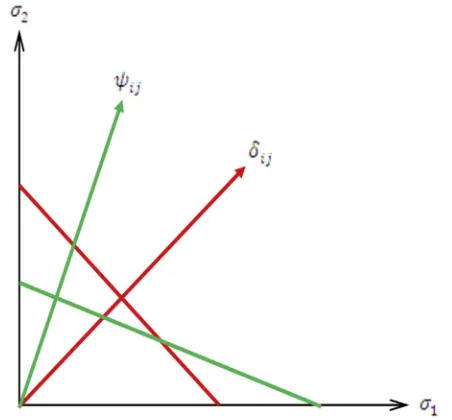
2.1. Representation in stress space

The representation of the new stress tensor decomposition in stress space is presented in this section. Bear in mind that any arbitrary stress state in stress space can be decomposed into hydrostatic and deviatoric parts. This representation which is applied for isotropic materials as shown in Eq. (7) is best presented in 3- and 2-dimensional stress spaces by red lines inFigs. 1 and 2with their directions perpendicular to each other. Recalling the new stress tensor decomposition, the representations of this decompositionψijin 3- and 2-dimensional stress spaces are shown inFigs. 1and2by green lines respectively. These figures represent the graphical interpretation of the generalized pressure axes of the new decompositionψijin 3- and 2-dimensional stress spaces respectively. From thesefigures, it can be observed that this decomposition leads to a shift of the pressure vector away from the common alignment (equal angle with the principal stress directions). Equally, it can be observed that the direction of the volumetric axisψij is not making the same angle with the principal stress directions. Based on the definition of the new stress tensor decomposition, any con-sidered orthotropic materials will uniquely define their own deviatoric plane within the stress space.

3. New constitutive model formulation

3.1. Kinematics forfinite strain deformations

The construction of the new hyperelastic-plastic constitutive model for orthotropic metals in this paper is based on the multiplicative decomposition of the deformation gradientF:

F F F= e p (8)

whereFeandFprepresent thermo-elastic part of the deformation and plastic part of the deformation (dislocation mechanics), respectively. This concept distinguishes the proposed constitutive model from hypoelastic-plastic material models (when elastic strains are small compared to the plastic strains). The intermediate (generally non-Euclidean) configuration corresponds to elastically unloaded material, known as the elastic reference configuration which can be physically obtained by elastic unloading of material (unstressed condition). The formulation based on additive decomposition of generalized strain measures is avoided in this work. As demonstrated by [36], this formulation leads to spurious shear stresses which are independent Fig. 1.ψ andδ as a vectors in a principal stress space. (For interpretation of the references to colour in thisfigure, the reader is referred to the web version of this article.)

of the elastic material properties for orthotropic materials. In addition, the evolution of material symmetry in orthotropic materials due to large deformations could not be tracked by the additive strain decom-position based model[37].

Using Eq. (8), the elastic right Cauchy-Green tensorCe and the elastic Green-Lagrange strain tensorEeare

C=F F∙ , E=1 C I F F I

2( − )= 1

2( ∙ − )

e Te e e e eT e ₍₉₎

The experimental work in[45]shows a strong correlation between elastic and plastic material symmetries. Therefore, the constitutive model described in this paper is developed and integrated in the isoclinic configuration. In other words, the hyperelastic part of the constitutive model is based on the assumption that the principal directions of material elastic and plastic orthotropy coincide and are not influenced by inelastic deformation. The requirements that free strain energy function is invariant under transformations of material symmetry and the non-uniqueness of the intermediate configuration are directly resolved by working in this configuration. This definition gives a significant simplification to the numerical implementation of the corresponding constitutive equations because one can steer clear of the explicit use of any corotational rate,[2]. To avoid confusion,(^)is used in this paper upon each of kinematic and kinetic variables defined with respect to the isoclinic configuration.

The structural tensorsMiii=1,2,3[11]are introduced to construct the orthotropy symmetric group ϑ. These tensors can be defined as

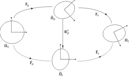
M1= ⨂n1 n1,M2=n2⨂n2 and M3= ⨂n3 n3 where n1,n2 and n3 are unit vectors represent an orthonormal frame of the material. By using the structural tensorsMˆiii= 1,2,3in the isoclinic configuration, the elastic free strain energy function for orthotropic materials considers the principal directions of material elastic orthotropy (material symmetry) in this configuration to be aligned with the unit (director) vectorsnˆ1,nˆ2 and nˆ3. As shown in Fig. 3, push forward transformations of the structural tensors from an initial configuration Ωo to elastically unloaded configuration Ωp can be defined as Mii=F M Fp ii −1p. The structural tensors Mii are pulled back from the elastically unloaded configuration (having an arbitrary orientation) Ωp to the isoclinic configuration Ωˆi by rotating back for plastically induced rigid body rotation due to plastic related deformations using below orthonormal transformation.

Mˆ =ii Q M QTp ii p (10)

whereQpis an orthonormal tensor that defines the rigid rotation due to plastic related deformation.

Referring to Fig. 3, a triad of unit vectors which represent the material symmetries is schematically shown by two orthogonal axes with arrows. Both elastic stretching and rotation are contained in the elastic partFe of the deformation gradientF. Plastic part ofF with respect to Ωp and Ωˆi is represented by Fp andFˆp respectively. The

plastic rotationRpis assigned toFpto ensure there is no rotation to the material principal axes of orthotropy (remainsfixed or unaltered by plastic deformation) in the isoclinic configurationΩˆi.

As examined in[64], the rotation and distortion during elastoplas-tic deformation are contained in the elaselastoplas-tic part ofF as a result of isoclinic configuration. Despite of general incompatibility tensorfields between elastic and plastic deformations, the elastic deformation may incidentally be compatible with plastic deformation when plastic or elastic deformation is homogeneous [64]. Alternatively, the plastic rotationRp can be assigned to the deformation due to damageFd to defineF F F Rˆ =e e d p if one considers the elastic material parameters to evolve due to damage since the changes of material compliance due to damage [71]. This assumption however not considered in this work.

The elastic and plastic parts of the deformation gradientF of the proposed constitutive formulation then can be defined explicitly in the isoclinic configuration as:

F Fˆ = , ˆ =e e Fp R FTp p=R R UTp p p=Up (11)

where plastic rotationRpis an orthogonal rotation tensor induced by plastic deformation and Up refers to plastic right stretch tensor. Subsequently, the total velocity gradient Lˆ can be decomposed additively into elasticLˆeand plasticLˆp parts. The incompressibility constraint is assumed to hold for plastic deformation which therefore gives

det F( ˆ )=1p (12)

3.2. Mandel stress tensor

In general, the Mandel stress tensorΣcan be defined as follows [46]:

S

Σ C= ∙ (13)

whereCandSrefer to Right Cauchy-Green tensor and Second Piola Kirchhoffstress tensor respectively. These tensors can be expressed in the elastically unloaded intermediate configurationΩpas

Ce=F Fe∙

T

e (14)

S=Fe∙ ∙τFe T

−1 −

(15)

The Kirchhoff stress tensorτ in Eq. (15) is a symmetric tensor defined in the current configurationΩtas

τ J= ∙ =σ det F σ( )∙ (16)

whereJis a volume ratio. Substituting Eqs.(14) and (15)into Eq.(13), the Mandel stress tensor in the intermediate configurationΩpcan be defined as

τ

Σ F= eT∙ ∙Fe−T=det F F σ F( )∙ Te∙ ∙ −eT (17) The Mandel stress tensor defined in Eq.(17)is frequently used to describe the behaviour of plastic materials[33]. This stress tensor is adopted in this work to formulate the new constitutive model for orthotropic metals. Choosing the isoclinic configurationΩˆias a point for integration, the Mandel stress tensor can be rewritten as

τ

Σ Fˆ = ˆ ∙ ∙ ˆe F

T e

T −

(18)

Further, Eq.(17)also can be expressed as follows:

τ

Σ Fˆ = ˆ ∙ ∙ ˆ = ˆ ∙ det( )∙ ∙ ˆ =F F F σ F det F F( )∙ ˆ ∙ ∙ ˆe σ F

T e

T

e T

e T

e T

e T

− − −

(19)

Usingσ =ij Pδij+Sij, the above equation can be defined as

δ

P

Σ det F Fˆ = ( )∙ ˆ ∙ ∙ ˆe σ F =det F F( )∙ ˆ ∙( + )∙ ˆS F

T e

T

e T

e T

− −

(20)

The formulation of the new generalized pressure for orthotropic metals is introduced in Eq. (20):

⎛ ⎝

⎜ _ψψψ ψ⎞_⎠⎟

Σ det F Fˆ = ( )∙ ˆ ∙e S+σ ∙ ∙ ˆF

T

e T −

(21)

Eq.(21)can be further extended as

ψ ψψ ψ

Σ det F Fˆ = ( )∙ ˆ ∙ ∙ ˆe S F +det F F( )∙ ˆ ∙σ ∙ ∙ ˆF

T e T e T e T Σ deviatoric Σ − ˆ ′= − ˆ_p (22)

whereΣˆp denotes the volumetric part (pressure) of the new Mandel stress tensor. Focusing on the deviatoric part instead of a full stress tensor, the deviatoric part of the new Mandel stress tensor is given by

⎛ ⎝ ⎜ ⎞ ⎠ ⎟ ψ ψψ ψ

Σˆ ′ =det F F( )∙ ˆe σ−σ ∙ Fˆ

T

e T −

(23)

Finally the new deviatoric Mandel stress tensor defined in the isoclinic configurationΩi, can be written as

ψ ψψ ψ

Σˆ ′ = det( )∙ ˆ ∙ ∙ ˆF F σ F − det( )∙ ˆ ∙F F σ ∙ ∙ ˆF =det F F( )∙ ˆ ∙ ∙ ˆe S F

T e T e T e T e T e T Σ Σ − ˆ − ˆ − p (24)

It can be easily proven the deviatoric component of the new Mandel stress tensor Eq.(24)is traceless (deviator tensor). As asserted in [54], existing experimental evidence shows that it is hard to deduce sound data about a continuum elastic domain for the skew-symmetric part of the Mandel stress tensor Σa. Much effort still required in terms of experimental work to establish the elastic domain and yield functions for the skew-symmetric part of the Mandel stress tensor. Therefore, in this work, only the symmetric part of the Mandel stress is considered [59,74].

A thermodynamics analysis presented inSection 3.6is based on the second law in the form of Clausius–Plank (CP) inequality, defined in the isoclinic configurationΩˆi. In order to define the CP inequality, it is necessary to introduce relevant conjugate variable pairs, starting with the stress power7.

7= :τ L det F σ L= ( )∙ : = : ̇ = ˆ ′: ˆS E Σ Lp (25) The stress power characterizes the real mechanical power during dynamic process. The representation of stress power is the product of work conjugate stress and strain measures. This thermodynamic part of the constitutive model is further discussed inSection 3.6.

3.3. Coupling of the proposed stress decomposition with equation of state EOS

In recent decades, the topic related to shock wave propagation in anisotropic materials has received considerable attention in the isotropic solid-state physics and mechanics literature [18,19,21,3,50,75,78]. Appropriate constitutive equations to describe the strength effect and the equation of state must be investigated to describe the anisotropic material response under shock loading. Therefore, in this work, the formulation is combined with an equation of state (EOS) in addition to the conservation laws to mathematically describe the material’s nonlinear behaviour and propagation of strong shock waves in solids due to shock loading.

An EOS represents a closure equation, which completes the relationships between the state variables in front of and behind a shockwave. Theoretically, the relationship described by EOS can be determined from the thermodynamic properties of the material, and require no dynamic data. However, practically, extensive dynamic experiments such as the planar shock wave experiment are required to characterize data on the material’s behaviour at high strain rates. In contemporary hydrocodes EOS’s are either of an analytical or a tabulated type. In this paper a very popular EOS that is extensively used for solid continua, the Mie-Gruneisen EOS[69,28], implemented in DYNA3D, is used. This an analytic EOS frequently used with solid materials. It defines the pressure as a function of densityρor specific

volume and specific internal energyeas shown below

P f ρ e p v v e e

v v

= ( , )=_r( )+ ( )( − ( ))r

ᴦ

(26)

wherevis the specific volume, (v)is the Grunesien gamma defined as

⎛ ⎝ ⎜ ⎞ ⎠ ⎟ P e v v ( )= ∂

∂ _{v (27)}

Generally is defined as constant =ᴦ0, or assumed that_v0= =const_v 0

ᴦ ᴦ

alternatively. The functionsp_randerare considered known functions of

von some reference curve. There are few possible reference curves to name such as the shock Hugoniot curve, the 0 °K isotherm, etc. However the most widely adopted form of the Mie-Gruneisen equation of state for solid materials which uses the shock Hugoniot as the reference curve is defined as follows

⎛ ⎝ ⎜ ⎞_⎠⎟

P f ρ e= ( , )=p ∙ + 1− μ ρ e 2 + H

ᴦ

ᴦ

(28)

where pH refers to Hugoniot pressure,μ= −1 ρ

ρ₀ is relative change of volume, is Gruneisen parameter, ρis density ande is the specific internal energy. The Rankine–Hugoniot equations for the shock jump conditions can be regarded by defining a relation between any pair of theρ,P,e,up(the velocity of the particle directly behind the shock) and U (the velocity of shockwave that propagates through the medium). There is an empirical linear relationship betweenU andupfor many liquids and most solids:

U c Su= + p (29)

wherec is the intercept of theU−up curve (U-shock velocity vs.up particle velocity curve), and S is the coefficient of theU−up curve slope. The Hugoniot pressure and a shock velocity normallyU are normally defined as a non-linear function of particle velocityup as follows[69]:

⎛ ⎝ ⎜ ⎞ ⎠ ⎟ ⎛ ⎝ ⎜ ⎞ ⎠ ⎟

U c S u S u U u S

u U u = + 1 p+ 2 p p+ 3 p p

2

(30)

The Gruneisen’s gamma for the undeformed materials can be expressed by γ au u = + 1 + 0 (31)

Hence, the pressure as a function of Gruneisen equation of state with cubic shock velocity can be defined as

⎡ ⎣ ⎢ ⎛_⎝⎜ ⎞_⎠⎟ ⎤ ⎦ ⎥ ⎡ ⎣ ⎢ ⎤ ⎦ ⎥

P μ Γ E μ

P ρ c μ μ Γ E μ

= + (1 + ) when > 0

= + (1 + ) when < 0

EOS

ρ c μ μ μ

S μ S S

EOS

1 + 1 − −

1 − ( − 1) − −

0 2 Γ Γ μ μ μ μ 02 _{2 2} 2

1 2 2 + 1 3

3 ( + 1)2

2

(32)

where

Eis the internal energy per initial specific volume,

S1, S2, S3are the coefficients of the slope of theU−upcurve, γ₀is the Gruneisen gamma for the un-deformed material, ais thefirst order volume correction toγ₀,

c S, 1, S2, S3, γ a ρ0, , 0 represent the material properties supplied by the user to characterize this EOS.

The combination between the proposed stress tensor decomposi-tion and the Mie-Gruneisen EOS requires some modifications to reflect the formulation of the generalized orthotropic pressure. Briefly,ψ is calculated using the material stiffness matrixCread from the inputfile. The increment of deviatoric Mandel stress tensorΣˆ ′is then calculated using rate of deformation tensorD. By setting pressure equals toPEOS, P P∼=EOS, the stress update at timen+ 1can be defined as

σn = ˆ′Σn −P ψ EOSn

+1 +1 +1

3.4. Orthotropy of elastic free energy function

To model the behaviour of orthotropic metals within elastic and plastic regimes the formulation of orthotropic tensor functions is constructed as a free strain energy function and a plastic level set function (orthotropic yield criterion). These tensor functions are defined fundamentally based on the representation of isotropic tensor functions theory. As aforementioned, a material symmetry groupϑis defined in this work to develop anisotropic tensor function for orthotropic constitutive behaviour. This orthotropic symmetric group is assumed to be unchanged during plastic deformation. Furthermore, the isotropic tensor function must be invariant under the special orthogonal group[20].

The elastic orthotropy of the proposed formulation is defined using the Helmholtz free energy as a function of evolving structural tensors. The Helmholtz free energy in the isoclinic configurationΩˆiis additively decomposed into elastic and plastic parts as

Ψ Ψˆ = ˆ ( ˆ )+ ˆeEe Ψp isot( )( )α (34)

In the above expression,Ψˆ ( ˆ )eEe represents the energy stored due to elastic deformations defined in terms of Elastic Green-Lagrange strain tensor Eˆe. In addition, Ψˆp isot( )(α) represents energy resulting from isotropic plastic hardening, whereαis the isotropic hardening variable (i.e. accumulated plastic deformation). The response of elastic material in the isoclinic configuration must be invariant under transformations of the material symmetry group ϑ. This is necessary based on the definition of isotropic functions.

Ψˆ (eQ E QTˆe )= ˆ ( ˆ ),∀ ∈ , ˆΨeEe Q ϑ Ee (35) whereQis orthogonal rotation tensor.Ψˆeis then known as aϑ-invariant function. Using the structural tensorsMˆii, the elastic component of free energy function for orthotropic materials can be expressed in terms of isotropic function in the isoclinic configuration as follows:

Ψ Ψˆ = ˆ ( ˆ , ˆ , ˆ )= ˆ ( ˆe eEe M11 M22 ΨeQE Qe T, QM Qˆ11 T, QM Qˆ22 T) (36) Ψˆecan be further defined in terms of a set of invariants of the Elastic Green-Lagrange strain tensorEˆe[20]such as

J1=trEe, J2= [(tr Ee) ], J= [(tr Ee) ] 2

3 3

m m m ₍₃₇₎

Using structural tensors that reflect the material symmetry of orthotropic materials, the irreducible invariants and the additional pseudo-invariants in the isoclinic configurationΩˆican be expressed as follows[79,65,20]etc.

J tr

J4= [tr M E11 e], J5= [tr M11(Ee) ], J= [tr M Ee], = [M (Ee) ] 2

6 22 7 22

2

m m m m

n n n n ₍₃₈₎

Subsequently, the elastic free energy functionΨˆecan be expressed in a quadratic form as

V V V V V V V J J J J J J

Ψˆ =1λJ μJ J J J J 2 + +

1

2 +

1

2 +2 +2 + + +

e 12 2 1 42 2 62 3 5 4 7 5 4 1 6 6 1 7 4 6 ₍₃₉₎

whereλ μ, , Vi i=1,..7in this case represent material parameters for the elastic orthotropic material. The second Piola-Kirchhoffstress tensorSˆ

in the isoclinic configurationΩˆi can be derived as Sˆ= Ψ E ∂ ˆ ∂ ˆ e

e, while the constant fourth-order tensorˆ is obtained by the second derivative of Ψˆe. Eventually the constant fourth-order tensorˆ that consists of the structural tensorsMˆiii=1,2,3can be defined in the isoclinic confi gura-tionΩˆias

V

V V V

V V V

λI I μ M M M M

M I I M M I I M

M M M M

ˆ = ⨂ +2 + ˆ ⨂ ˆ + ˆ ⨂ ˆ +2 +2

+ ( ˆ ⨂ + ⨂ ˆ )+ ( ˆ ⨂ + ⨂ ˆ )+

( ˆ ⨂ ˆ + ˆ ⨂ ˆ )

1 11 11 2 22 22 3 1 4

2 5 11 11 6 22 22 7

11 22 22 11

  



(40)

where

δ δ

δ δ

δ δ M M

M M

= = (fourth − order unit tensor) = ˆ + ˆ ,

= ˆ + ˆ

ik jl jl ik

ik jl jl ik

ijkl ik jl 1

1 1

2

2 2

  

 ₍₄₁₎

Note that the conventional relation between stress and strain tensor in the isoclinic configurationΩˆican be expressed as follows:

Sˆ =ˆij ijklEˆkl (42)

whereijklis a fourth-order elasticity or material stiffness tensor. This tensor can be set equal toˆ to defineλ μ, , Vi i=1,..7with respect to the elasticity orthotropic parameters. By choosing the preferred directions asn=[1,0,0]T

1 andn2=[0,1,0]T, the new elastic orthotropic constants can be defined as follows

V

V V

V V V V

λ= +2( − − ) =μ + − = + −4 −2 = + −

4 −2 = − = − = − −2( − − ) = −

−2( − − ) = − − + +2( − − )

33 44 55 66 55 66 44 1 11 33 55 13 2 22 33

66 23 3 44 66 4 44 55 5 13 33 44 55 66 6 23 33

44 55 66 7 12 13 23 33 44 55 66

            

            

          (43)

3.5. Orthotropic yield criterion

The aim of yield function formulation is to model plastic anisotropy by using the structural tensors defined in terms of isotropic function of the material symmetry group ϑ. In the proposed formulation, the orthotropic yield function is defined using the classical Hill’s yield criterion[29]. The hardening is modelled as an isotropic hardening. Therefore, the yield surface is expected to maintain its initial shape (change in size, not shape). The yield surface expansion is controlled by the physically and a thermally micromechanical-based model– Mechanical Threshold Stress (MTS) model[24].

The dependence on material anisotropy during plastic deformation is modelled by the introduction of the structural tensors Mˆiii=1,2,3 with respect to the isoclinic configurationΩˆi. The corresponding yield surface is defined in a new deviatoric plane as a result of the new stress tensor decomposition. Using the symmetric Mandel stress tensor defined in Eq.(24), the yield function can be written as

fˆ =ˆ ( ˆ ′, )f Σ α (44)

whereαis an isotropic hardening variable. The properties of symmetric orthotropy are considered by introducing the structural tensors,Mˆiias follows:

fˆ =ˆ ( ˆ ′, ˆ , )f Σ Mii α (45)

Accordingly, the plastic anisotropy of the new constitutive model is characterized by Hill’s anisotropy yield function as follows:

fˆ = ˆ ′: ˆ : ˆ ′ − ˆ ( )=0Σ  Σ f α (46) where_ˆ _{is a fourth-order tensor defined in the isoclinic configuration}

Ωˆi. The dependence of the above yield function on Hill’s yield criterion and structural tensors is represented by this tensor. fˆ (α)in the above equation defines the evolvingflow stress that is controlled by isotropic hardening. The Hill’s effective stress can be expressed in terms of the deviatoric Mandel stress in the isoclinic configurationΩˆias follows:

⎡

⎣ ⎢ ⎢ ⎢ ⎢ ⎢ ⎢

⎤

⎦ ⎥ ⎥ ⎥ ⎥ ⎥ ⎥

F G H L

M N

F G H

Σ

Σ Σ Σ Σ Σ Σ Σ

Σ Σ

ˆ ′ = 3 2

( ˆ ′ − ˆ ′ ) + ( ˆ ′ − ˆ ′ ) + ( ˆ ′ − ˆ ′ ) + 2 ˆ ′

+ 2 ˆ ′ + 2 ˆ ′

+ +

y z z x x y yz

zx xy

2 2 2 2

2 2

(47)

⎡ ⎣ ⎢ ⎢ ⎢ ⎢ ⎢ ⎢ ⎤ ⎦ ⎥ ⎥ ⎥ ⎥ ⎥ ⎥ G H H G H H F F G F F G N L M ˆ = + − − 0 0 0 − + − 0 0 0 − − + 0 0 0 0 0 0 2 0 0 0 0 0 0 2 0 0 0 0 0 0 2  (48)

By comparing the Hill’s matrix with the fourth-order isotropic tensor function _ˆ _{in Eq. (40) the orthotropic plastic constants}

V

λ μ

( , , i i=1,..7)are obtained:

V V

V V V V

V

λ F G N L M μ L M N F H G L G

H F M N M N L F G L M N G

F L M N H F G N L M =1

2 + 1

2 +2( − − ) = + − = 1 2 +

1

2 +2 −4 = 1 2 +

1 2

+2 −4 = − = − =−1

2 – +2 +2 −2 =− 1 2 –

+2 +2 −2 =−1

2 + + +2 −2 −2

1 2

3 4 5 6

7 ₍₄₉₎

3.6. The Clausius-Plank inequality

The evolution equations for the specified variables of the new constitutive model are defined with respect to the second law of thermodynamics framework. Using the Clausius-Plank inequality, an isothermal and uniform temperature distribution type of deformations can be expressed as

+=S: Ė − ̇≥0Ψ (50)

whereΨ̇ is a rate of Helmholtz free energy function, andĖ is

Ė =1C

2

̇

(51)

Using Eqs.(51)and(50)can be rewritten as follows:

+= :S 1C Ψ

2 ̇ − ̇ ≥0 (52)

Considering the free strain energy (Helmholtz free energy) function is represented by the elastic Cauchy-Green strain tensorCe, and the strain-like internal variable describing isotropic plastic hardeningξ_h,

ξ

Ψ Ψ= (Ce, h), this function can be easily divided into elastic and plastic as

Ψ Ψ= e(Ce)+Ψ ξp( )h (53)

The differentiating of the above equation with respect to time leads to

Ψ Ψ Ψ

ξ ξ C C ̇ =∂ ∂ : ̇ + ∂ ∂ ∙ ̇ e e e p h h (54)

Substituting Eq.(54)into Eq.(52)gives

+ ⎛

⎝

⎜ ⎞

⎠ ⎟

S Ψ Ψ

ξ ξ

C

C C

= : 1 2 ̇ −

∂ ∂ : ̇ +

∂ ∂ ∙ ̇ ≥0 e e e p h h (55)

Using Ce=Fp ∙ ∙C F

T p

− −1 _{and its material time derivative}

Ċ = ̇ ∙ ∙e Fp C F +F ∙ ̇ ∙C F +F ∙ ∙ ̇C F

T

p pT p pT p

− −1 − −1 − −1

, the Mandel stress tensor can be expressed as:

⎛ ⎝

⎜ ⎞_⎠⎟

S Ψ Ψ

Σ C F C F F

C F C C

= ∙ =( ∙ ∙ )∙ 2∙ ∙∂

∂ ∙ =2∙ ∙ ∂ ∂ p

T

e p pT e

e

p e e

e

− −1

(56)

Using Eq. (56), the non-negative of the internal dissipation can finally be defined as follows:

+ Ψ

ξ ξ

Σ L

= : −∂ ∂ ∙ ̇ ≥0 p

p

h h

(57)

The evolution equations for the plastic strain tensors are derived based on the principle of maximum plastic dissipation. In addition, the normality rules gives function ofLpandξḣ as

f

ξ f

L λ

Σ λ α

= ̇ ∂ ∂ ′, ̇ = ̇

∂ ∂

p h ₍₅₈₎

These equations satisfy the associativeflow rule and the expression for evolution equation, respectively. Equallyξ̇

h is a work conjugate of the stress-like internal variable describing isotropic hardening α. Finally the local dissipation inequality can be expressed with respect to the isoclinic configurationΩˆias

+ˆ = ˆ ′: ˆ − : ̇ ≥0Σ Lp α ξh (59) where

f

ξ f

L λ λ

α =⋅ ∂ ∂Σ′, ⋅ =⋅ ∂ ∂ h P _l

m l l

(60)

Since the Mandel stress adopted in the formulation is symmetric and because this stress measure is thermodynamically conjugate to the plastic velocity gradient, only the symmetric part of the plastic velocity gradient is adopted in the formulation. Therefore, in this work, the plastic spin is assumed vanish in the chosen isoclinic configuration. Using symmetry of Mandel stress and assuming that the plastic spin is equal to zero in the isoclinic configurationΩˆi, Eq.(59)can be rewritten as

+ˆ = ˆ ′:Σ symLˆ − : ̇ ≥0p α ξh (61) The above expression is also written as

+ˆ = ˆ ′: ˆ − : ̇ ≥0Σ Dp α ξh (62) A similar approach has been adopted in[20], in contrast to the concept used by[61–63]that define a so-called plastic material spin. By using the yield function Eq.(46)in thefirst part of Eq.(60), the evolution of the plastic deformationDˆpcan be expressed as follows:

D λ Σ Σ Σ Σ

Σ Σ

ˆ = ̇( ˆ ∙ ˆ ′+( ˆ ∙ ˆ ′) + ˆ ∙ ˆ ′+( ˆ ∙ ˆ ′) ) 4 ˆ ′: ˆ : ˆ ′

p

T T T T

   

 (63)

Therefore, the inequality of dissipation energy in Eq.(62)can be expressed as follows:

+ ⎡ ⎣ ⎢ ⎢ ⎤ ⎦ ⎥ ⎥ ξ

Σ λ Σ Σ Σ Σ

Σ Σ

α

ˆ = ˆ ′∙ ̇( ˆ ∙ ˆ ′+( ˆ ∙ ˆ ′) + ˆ ∙ ˆ ′+( ˆ ∙ ˆ ′) ) 4 ˆ ′: ˆ : ˆ ′

− : ̇ ≥0

T T T T

h

   

 (64)

Using the above identities, eventually the Clausius-Plank inequality of the second law of thermodynamics for the new constitutive model can be expressed with respect to the isoclinic configuration Ωˆi as follows: + ⎛ ⎝ ⎜ ⎞ ⎠ ⎟ f

λ Σ Σ α

α

ˆ = ̇ ˆ ′: ˆ : ˆ ′ − : ∂ ∂ ≥0 

(65)

3.7. Plasticflow rule of the new constitutive model

The evolution equation which determines the relation between the stress and strain increments of the constitutive relations is defined from the consistency condition. Let usfirst write the plastic velocity gradientLˆpin the isoclinic configurationΩˆias

Lˆ = ˆ̇ ∙ ˆ =λ̇ˆ ( ˆ ′, α)p F Fp p r Σ

−1

(66)

The plasticflow direction is marked by rˆ and set equal to f Σ ∂ ˆ ∂ ˆ ′. Further, the evolution of isotropic hardening law is given by

H Σ

α̇=λ̇ ˆ ( ˆ ′, α) (67)

consistency condition of the new constitutive model can be defined as

fˆ ̇=ˆ ,: ˆ̇′ + ˆ ∙ ̇=0fΣˆ Σ fα α (68)

where

f f f f

Σ α

ˆ ′=

∂ˆ ∂ ˆ ′ˆ =

∂ˆ ∂

Σˆ α

(69)

Using Σˆ ′ = 3( ˆ ′ ˆ ) ˆ ′Σ TΣ

2  to define the orthotropic yield criterion, fˆ (α)in Eq.(46)can be re written as

fˆ ( ) =α 2Σ

3ˆ ′ (70)

The rate of this expressionα̇can be expressed as

α̇ = 2Σ

3 ˆ ′ ˙

(71)

whereΣˆ ′

˙

is given by

Σˆ = ˆ ˆHDp ˙ ′

(72)

Combining Eqs.(71) and (72)results in

α⋅ = 2HD

3 p

l l

(73)

Subsequently, simplifying 2Hˆ

3 asK

ˆ

f and definingDˆ =p 2λ̇ 3 , the above equation can be rewritten as

α λ̇= ̇ 2K

3 ˆ_f

(74)

Using this equation, the consistency condition of the new constitu-tive model Eq.(68)can be re expressed as

fˆ ̇=ˆf Σ f λ K

′: ˆ

̇_{′ + ˆ ∙ ̇} 2 3 ˆ =0f

Σˆ α

(75)

The formulation of the plasticflow equation in the intermediate configuration requires the decomposition of the deformation rate into elastic and plastic parts. The formulation however differs between hyperelastic-plastic materials defined in this work and hypoelastic-plastic materials when the hypoelastic-plasticflow equation is specified in terms of plastic velocity gradientLˆp as shown in Eq.(66), [10]. Subsequently, usingΣˆ̇′=_E∂ ˆΨ_E : ˆĖe=CΣel : ˆĖe=CelΣ :( ˆ − ˆ )D Dp

∂ ˆ ∂ ˆ

ˆ ˆ

e e

D D

2

in the above equation where

Cel=

Ψ Σ

E E

ˆ ∂ ˆ

∂ ˆ ∂ ˆ D

e e

2

refers to the elasticity tensor (material stiffness tensor) that

relates the material time derivative of the Mandel stress Σˆ̇′ to the material time derivative of the Green strain Eˆ̇e in the isoclinic configurationΩˆi, the consistency condition of the proposed formulation in the isoclinic configurationΩˆican be further derived as follows:

fˆ ̇=ˆf C D D f λ K

′: :( ˆ − ˆ )+ ˆ ∙ ̇ 2 3 ˆ

el p f

Σ Σ α ˆ ˆ_D (76)

IntroducingDˆpequals tosym ˆ =λ̇symˆLp rin the above equation,[10], the plastic rate parameterλ̇can be expressed as

f

f f

λ C D

K C symr

̇= ˆ ′: : ˆ − ˆ ∙ ˆ + ˆ

′: : ˆ el f el Σ Σ α Σ Σ ˆ ˆ 2 3 ˆ ˆ D D (77)

3.8. The Elasto-Plastic tangent modulus

The plastic rate parameterλ̇ can be used to explicitly define the relation between the stress and strain increments of the new constitu-tive model in the isoclinic configurationΩˆi within elastic and plastic

regimes using the following equation:

Σˆ̇ ′ =C_el :( ˆ − ˆ )=D Dp Cel :( ˆ − ̇D λsymrˆ)

Σˆ_D Σˆ_D

(78)

Using Eq.(77), this equation can be further written as follows:

⎛ ⎝ ⎜ ⎜⎜ ⎞ ⎠ ⎟ ⎟⎟ f f f

Σ C D C D

K C symr

symr

ˆ̇ ′ = : ˆ −

ˆ

′: : ˆ − ˆ ∙ ˆ + ˆ

′: : ˆ ˆ el el f el Σ Σ Σ α Σ Σ ˆ ˆ ˆ 2 3 ˆ ˆ D D D (79)

Finally, with some arrangements the relationship between the stress and strain increments within elastic and plastic regimes inΩˆi is concluded by the elasto-plastic tangent modulusC

′ Σˆ;

f

f f

C C C symr C

K C symr

′= ′−

( : ˆ) ⊗ ( ˆ ′: ) − ˆ ∙ ˆ + ˆ

′: : ˆ

el el el

f el Σ Σ Σ Σ Σ α Σ Σ ˆ ˆ ˆ ˆ ˆ 2 3 ˆ ˆ D D D (80)

4. Validation and results

The proposed formulations in the preceding sections are imple-mented into the LLNL-DYNA3D and named Material Type 93. On the completion of the implementation process, the capability of the new constitutive model to capture strain rate and temperature sensitivities of orthotropic materials is first checked. The numerical simulation results of the newly proposed constitutive model are then compared against the published experimental data of Plate Impact and Taylor Cylinder Impact Tests A cm−g−μs units system is adopted in the involved numerical tests.

4.1. Strain rate and temperature dependency tests

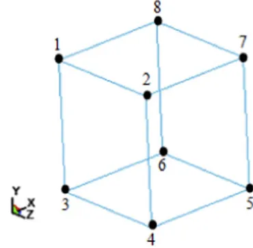
To investigate rate sensitivity and temperature sensitivity of the new constitutive model, a series of one element analyses are per-formed. The single element with the node numbering used to define boundary conditions is shown inFig. 4. Assuming the single element represents one of the elements around the gauge length of the uniaxial stress test’s specimen, the uniform plastic deformation observed in the element is applicable to predict strain rate and temperature dependent using this simplified analysis. Bear in mind that this comparison method is only valid for the test data before the plastic deformation occurs non-uniformly (localisation or necking) in the test specimen.

In this model the principal directions of material orthotropy are aligned with the x y z, , axis of the global coordinate system. The displacement boundary conditions applied in these tests are sum-marised inTable 1. Loading in tension is applied to the elements by

prescribing displacement load curves to nodes 1, 2, 3 and 4.

The tensile test data of Aluminium 7010 published in[56]is used in this validation stage. The parameters defined for this specimen are given inTables 2and3.

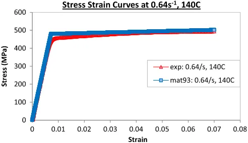
The stress-strain curves for quasi-static tension tests (6.4x10−4 −1s _{strain rate) conducted at−50 °C and70 °Care presented} in Fig. 5. In addition, Fig. 6 shows the stress-strain curves of the specimen tested at140 °Cat two different strain rates;6.4x10 s0 −1_and 6.4x10−1 −1s _{. It can be clearly seen from thesefigures that the specimen} exhibits strain rate and temperature sensitivity.

The strain rate and temperature predictions of the newly constitu-tive model are shown in the followingfigures.

Figs. 7–10 show that the flow stress (MTS model) of the new constitutive model shows a good agreement with the rate and temperature sensitivity of the specimen. The flow stress formulated as a function of the microstructural state has captured a reasonable relationship between stress, strain rate and temperature of Aluminium 7010. Small variances between the simulation and the experimental results might be caused by the MTS properties used to control theflow stress of the new constitutive model.

It can be concluded that increasing strain rate increases theflow stress, while increasing temperature decreases theflow stress. In other words, the saturation stress of the new formulation increases with

increasing strain rate and decreases with increasing temperature.

4.2. Plate impact test analysis of aluminium alloy 7010

The capability of the newly implemented constitutive model to represent the behaviour of orthotropic metals when impacted with shock loading at high impact velocity is investigated in this stage. Fig. 11shows the configuration of the Plate Impact test simulation. Table 1

Displacements boundary condition for a uniaxial stress and uniaxial strain tests in thex

direction.

Node number Displacement boundary condition of uniaxial stress

1 No constraints

2 No constraints

3 No constraints

4 No constraints

5 Constrainedx y, andzdisplacements

6 Constrainedxdisplacement

7 Constrainedxdisplacement

8 Constrainedxdisplacement

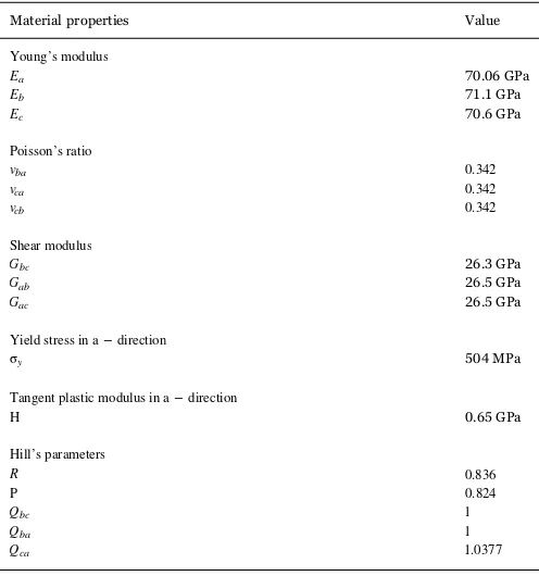
Table 2

Aluminium 7010 material parameters for elastic-plastic with isotropic plastic hardening analysis.

Material properties Value

Young’s modulus

Ea 70.06 GPa

Eb 71.1 GPa

Ec 70.6 GPa

Poisson’s ratio

vba 0.342

vca 0.342

vcb 0.342

Shear modulus

Gbc 26.3 GPa

Gab 26.5 GPa

Gac 26.5 GPa

Yield stress in a − direction

σy 504 MPa

Tangent plastic modulus in a − direction

H 0.65 GPa

Hill’s parameters

R 0.836

P 0.824

Qbc 1

Qba 1

Qca 1.0377

Table 3

MTS parameters of aluminium 7010.

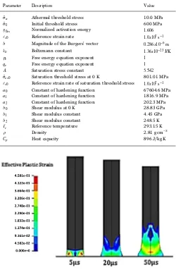
Parameter Description Value

σˆa Athermal threshold stress 100 MPa

σˆ0 Initial threshold stress 600 MPa

g0εs Normalized activation energy 1.606

εṡ0 Reference strain rate 1.0 10 sx 7 −1

b Magnitude of the Burgers’vector _{0.286 10x} −9_m

kb Boltzmann constant 1.36 10x −23J/K

pε Free energy equation exponent 1

qε Free energy equation exponent 1

A Saturation stress constant 5.542

σˆεs0 Saturation threshold stress at 0 K 801.01 MPa

εṡ0 Reference strain rate of saturation threshold stress 1.0 10 sx 7 −1

a0 Constant of hardening function 67604.6 MPa

a1 Constant of hardening function 1816.9 MPa

a2 Constant of hardening function 202.3 MPa

b0 Shear modulus at 0 K 28.83 GPa

b1 Shear modulus constant 4.45 GPa

b2 Shear modulus constant 248.5 K

Tr Reference temperature 293.15 K

ρ Density 2.81 g cm−3

Cp Heat capacity 896 J/kg K

Fig. 5.Stress Strain Curves of Aluminium 7010 at6.4 10x −4 −1s _{at different temperatures.}

0 100 200 300 400 500 600

0.00 0.02 0.04 0.06 0.08 0.10 0.12 0.14 0.16

Stress (MPa)

Strain

Stress Strain Curves of Al7010 at Different Strain

Rates

exp: 6.4/s, 140C exp: 0.64/s, 140C

It can be observed that the test consists of three parts of rectangular bars with4 4x solid elements for its cross section (XYplane). Thefirst bar represents the PMMA block, while the second and third bars refer to the test specimen andflyer respectively. The mesh of this simulation is set to allow a 1D wave to propagate along the length of the bars when the impact happens. From this figure, it is noticed that symmetrical planes are adopted on all sides of the bars.

To ensure that no release wave is reflected from the back of the PMMA block into the test specimen, a non-reflecting boundary condition is applied to the back of this block (PMMA). In addition, theflyer, test specimen and PMMA bars are modelled with 25 solid elements (2.5 mm in length), 75 solid elements (10 mm in length) and 100 solid elements (12 mm in length) respectively, parallel to the impact axis (Zaxis). A contact interface is defined in between theflyer

and the test specimen. To record the stress time histories of the impact, a time history block is defined in the elements at the top of PMMA bar. In this analysis, the longitudinal stress (Z stress) in the elements at the top of the PMMA bar is compared with the experimental data with respect to the short transverse and the longitudinal (rolling) directions of the specimen. The MTS flow stress is excluded at this stage of validation. The material properties used in this analysis are shown in Table 4.

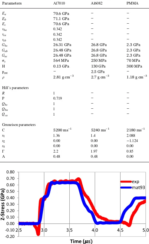
Theflyer is defined as Aluminium6082−T6. Both theflyer and the PMMA blocks are assigned with DYNA3D’s Material Type 10 (Isotropic-Elastic-Plastic-Hydrodynamic). The Gruneisen equation of state is adopted to appropriately represent the shock loading developed in this test. In addition, three different impact velocities are performed in these analyses 234 ms−1_{, 450 ms}−1 _{and 895 ms}−1_{. By setting the} material axes definition as AOPT 2 (globally orthotropic), the following results are obtained:

It can be observed inFigs. 12–17that the elastic-plastic loading-unloading behaviours of theAl7010are well captured by the proposed constitutive model. A slope that is developed in the initial increment of the longitudinal stress represents the Hugoniot Elastic Limit (HEL). Without knowing the error that might happen in the experimental test, such as an inaccuracy of the gauge used to measure the longitudinal stress etc., a slight difference between the new constitutive model’s HEL and the values obtained experimentally is acceptable. In addition, a different HEL value obtained in each direction is a sign of an adequate anisotropy level of the material under consideration.

The width of the generated pulses in each analysis is reasonably agreed with the experimental test data. Furthermore, very close Hugoniot stress levels between the new constitutive model and the experimental data proved the capability of the newly implemented orthotropic pressure to capture shockwaves in orthotropic materials. The comparison between Material Type 93 and the experimental results are analyzed and summarised inTable 5.

In this analysis, it can be clearly seen that the tensile wave failure or Fig. 7.Stress strain curves comparison between Mat93 and experimental data at

x

6.4 10−4 −1s _{,−50 °C.}

Fig. 8.Stress strain curves comparison between Mat93 and experimental data at 6.4x10−4_{s, 70 °C.}

0 100 200 300 400 500 600

0.00 0.01 0.02 0.03 0.04 0.05 0.06 0.07 0.08 0.09

Stress (MPa)

Strain

Stress Strain Curves at 6.4 s

_{, 140}

_°

_C

exp: 6.4/s, 140C mat93: 6.4/s, 140C

Fig. 9.Stress strain curves comparison between Mat93 and experimental data at 6.4x10−4_{s, 140 °C.}

Fig. 10.Stress strain curves comparison between Mat93 and experimental data at 6.4x10−4_{s, 140 °C.}

V

PMMA

SPECIMEN

FLYER

spall (demonstrated by the reloading of the longitudinal stress after the first loading-unloading pulse) is not generated in the specimen when impacted with a lower impact velocity (234 ms−1_{). However, a clear} spall criterion can be observed when higher impact velocities (450 ms−1_{and 895 ms}−1_{) are applied. Such behaviour could not be} captured by the Material Type 93 due to the absence of damage and failure models in the proposed formulation of this constitutive model.

4.3. Taylor cyliner impact test analysis of aluminium alloy 7010

The capability of the new constitutive model to represent the deformation behaviour of orthotropic metals within a three-dimen-sional stress state is accessed in this section. A standard configuration of this simulation test is depicted byFig. 18.

It can be observed that this test creates an impact between a solid cylinder rod of material (specimen) and afixed rigid surface (anvil) as a target. Strictly speaking, a cylindrical rod isfired into afixed rigid plate at high velocity (left). This impact subsequently produces permanent Table 4

Material properties for plate impact test analysis.

Parameters Al7010 Al6082 PMMA

Ea 70.6 GPa − −

Eb 71.1 GPa − −

Ec 70.6 GPa − −

vba 0.342 − −

vca 0.342 − −

vcb 0.342 − −

Gbc 26.31 GPa 26.8 GPa 2.3 GPa

Gab 26.48 GPa 26.8 GPa 2.3 GPa

Gac 26.48 GPa 26.8 GPa 2.3 GPa

σy 564 MPa 250 MPa 70 MPa

H 0.13 GPa 130 GPa 300 MPa

pcut − 2.5 GPa −

ρ 2.81 g cm−3 _{2.7 g cm}−3 _{1.18 g cm}−3

Hill’s parameters

R 1 − −

P 0.719 − −

Qbc 1 − −

Qba 1 − −

Qca 1 − −

Gruneisen parameters

C 5200 ms−1 _{5240 ms}−1 _{2180 ms}−1

s1 1.36 1.4 2.088

s2 0.00 0.00 −1.124

s3 0.00 0.00 0.00

Г 2.2 1.97 0.85

A 0.48 0.48 0.00

Fig. 12.Longitudinal stress (Z stress) comparison at 234 ms−1_{in longitudinal direction.}

Fig. 13.Longitudinal stress (Z stress) comparison at 234 ms−1_{in transverse direction.}

Fig. 14.Longitudinal stress (Z stress) comparison at 450 ms−1_{in longitudinal direction.}

Fig. 15.Longitudinal stress (Z Stress) comparison at 450 ms−1_{in transverse direction.}

Fig. 16.Longitudinal stress (Z stress) comparison at 895 ms−1_{in longitudinal direction.}