Large sample properties of the three step euclidean likelihood estimators under model misspecification

(1)

Munich Personal RePEc Archive

Large sample properties of the three-step

euclidean likelihood estimators under

model misspecification

Dovonon, Prosper

Concordia University, CIREQ

18 November 2008

(2)

Large Sample Properties of the Three-Step Euclidean Likelihood

Estimators under Model Misspecification

Prosper DOVONON∗

Concordia University and CIREQ

First Draft: November 18, 2008

This Draft: May 16, 2010

Abstract

This paper studies the three-step Euclidean likelihood (3S) estimator and its corrected version as proposed by Antoine, Bonnal and Renault (2007) in globally misspecified models. We establish that the 3S estimator stays√

n-convergent and asymptotically Gaussian. The discontinuity in the shrinkage factor makes the analysis of the corrected-3S estimator harder to carry out in misspecified models. We propose a slight modification to this factor to control its rate of divergence in case of misspecification. We show that the resulting modified-3S estimator is also higher order equivalent to the maximum empirical likelihood (EL) estimator in well specified models and √

n-convergent and asymptotically Gaussian in misspecified models. Its asymptotic distribution robust to misspec-ification is also provided. Because of these properties, both the 3S and the modified-3S estimators could be considered as computationally attractive alternatives to the exponentially tilted empirical likelihood estimator proposed by Schennach (2007) which also is higher order equivalent to EL in well specified models and√

n-convergent in misspecified models.

Keywords: Misspecified models, Empirical likelihood, Three-step Euclidean likelihood.

∗_{I thank Yuichi Kitamura, and two anonymous referees for very helpful suggestions that led to a much improved}

(3)

1 Introduction

The lackluster performance of the generalized method of moments (GMM) estimator in finite samples

has paved the way for several competing alternative efficient estimators. Among them, maybe the

most known are the continuously updated GMM (CU) estimator proposed by Hansen, Heaton and

Yaron (1996) also known to be identical to the Euclidean empirical likelihood (EEL) estimator, the

maximum empirical likelihood (EL) estimator proposed by Qin and Lawless (1994) and the exponential

tilting (ET) estimator introduced by Kitamura and Stutzer (1997). These estimators are included in

both the minimum discrepancy (MD) class of estimators formulated by Corcoran (1998) and the

generalized empirical likelihood (GEL) class of estimators proposed by Newey and Smith (2004).

When comes to the comparison of these estimators, three points are considered as major issues. The

implementation cost, the finite sample bias and the behaviour under model misspecification. All these

alternative estimators are computationally very demanding. They are expressed as solutions of saddle

point problems and impose a double optimization program solving in their calculation process. (See

Kitamura (2006).) When a large parameter vector is considered, these saddle point problems are

computationally cumbersome. On the other hand, because of their one-step nature, these estimators

have a fewer sources of higher order (O(n−1)) bias than the efficient two-step GMM and, as shown by

Newey and Smith (2004), the EL estimator has even fewer higher order bias sources than all of the

other estimators. Still, this enjoyable property of the EL estimator holds only in correctly specified

models. A moment condition model is globally misspecified if the true data generating process deviates

from these moment conditions such that no value in the parameter space solves the population moment

conditions. In the case of global misspecification, Schennach (2007) establishes that EL ceases to be

√

n-convergent whereas ET is√n-convergent (Imbens (1997)) and CU may also be√n-convergent.

As one can notice, none of these regular estimators enjoys all of the desirable properties. The

most recent estimators proposed in the literature aim to combine several of them to deliver new

ones with better performance. Schennach (2007) combines the EL and ET estimators to propose

the exponentially tilted empirical likelihood (ETEL) estimator which is, in well specified models,

higher order equivalent to EL in the sense that their difference is of order Op(n−3/2) and is √n

-convergent in misspecified models. Still, the ETEL estimator is as computationally costly as both

EL and ET. Antoine, Bonnal and Renault (2007) combine the two-step efficient GMM estimator with

the Euclidean empirical likelihood implied probabilities to deliver the so-called three-step Euclidean

likelihood (3S) estimator. As these implied probabilities could be negative causing some instability

(4)

likelihood implied probabilities corrected by shrinkage. As highlighted in this paper through our Monte

Carlo simulations, such corrections to the implied probabilities are crucial to take any benefit from the

three-step procedure. In particular, the 3S estimator appears to be too sensitive to negative implied

probabilities and is computationally inefficient with too many outliers in such cases. Nevertheless,

these two estimators share two important advantages. They are computationally convenient and are

also higher order equivalent to the EL estimator in well specified models.

This paper studies the three-step Euclidean likelihood estimators under global misspecification.

Inference under misspecification is getting more and more attention in the econometric literature.

White (1982) studies the quasi maximum likelihood estimator when the distributional assumptions are

misspecified. Hall (2000) examines the implications of model misspecification for the heteroskedasticity

and autocorrelation consistent covariance matrix estimator and the GMM overidentifying restrictions

test. Hall and Inoue (2003) study the GMM estimators under global misspecification. Schennach

(2007) analyzes the EL and ETEL estimators under global misspecification while Kan and Robotti

(2008) propose a methodology to evaluate the Hansen-Jagannathan distance between two pricing

kernels in the case of model misspecification.

One of the main motivations for studying estimators in globally misspecified models is underlined

by Schennach (2007). Statistical models are only simplification of a complex reality and therefore are

bound to be misspecified. Specification tests aim to indicate the candidate models which seem closer

to the sample under studies and may be sharp to detect globally misspecified models. Nevertheless, it

is frequent to come across parsimonious models delivering better forecasting performances but failing

the specification tests while other less parsimonious models pass these tests with very poor

out-of-sample performance. For such parsimonious models, √n-convergent estimators are useful to allow

asymptotic approximations through usual sample sizes. Furthermore, the asymptotic behaviour of

these estimators also need to be fully derived.

In the context of moment condition-based models in particular, the specification tests for

overi-dentifying restrictions could validate the model. In the case of rejection, if no theory is available for

inference, empirical researchers could have to drop parsimonious, robust and competitive models for

forecasting for other less attractive. The situation could even be more ambiguous. Hall and Inoue

(2003) report several empirical researches in the literature in which inference by the usual asymptotic

distributions have been performed even though the data have rejected the overidentifying restrictions.

In this paper, we provide global misspecification robust inference for the 3S estimator. We show that,

in the case of moment misspecification, this estimator stays √n-convergent and is asymptotically

(5)

The main intuition behind this asymptotic behaviour of the 3S estimator under misspecification

is related to the fact that its estimating function is equivalent to a smooth function of sample means.

This is not the case for the corrected 3S estimator. The discontinuity in the shrinkage factor makes its

analysis more difficult. We establish that, under mild conditions, the shrinkage factor diverges such

that the estimating function can be considered as an approximation of a smooth function of sample

means. But, the asymptotic distribution derivation requires to control the rate of divergence of this

factor. For that purpose, we propose a slight modification of the original shrinkage factor proposed by

Antoine, Bonnal and Renault (2007) which simplifies the derivations. We call the estimator resulting

from the new shrinkage factor themodified three-step Euclidean likelihood (m3S) estimator. The m3S estimator is as easy to compute as the 3S estimator. Additionally, we show that in correctly specified

models the m3S estimator is higher order equivalent to both the EL and the 3S estimators. As the

m3S estimator is computed via implied probabilities corrected for the sign, it is more stable than the

3S estimator. We show that under global misspecification the m3S estimator stays √n-convergent

and asymptotically Gaussian. Its asymptotic distribution robust to global misspecification is also

provided. This makes both the 3S and the m3S estimators two computationally appealing alternative

to the ETEL estimator.

The remainder of the paper is organized as follows. Section 2 describes the model and the estimators

and establishes the higher order equivalence of the m3S and the EL estimators in well specified models.

In Section 3 we derive asymptotic results for the 3S and m3S estimators under moment misspecification.

Our Monte Carlo experiments are introduced in Section 4 followed by Section 5 which concludes. All

proofs are gathered in the Appendix.

2 The three-step Euclidean likelihood estimators

The statistical model that we consider in this paper is one with finite number of moment restrictions.

To describe it, let {xi :i= 1, . . . , n}be independent realizations of a random vector x and ψ(x, θ) a

knownq-vector of functions of the data observationxand the parameterθwhich may lie in a compact

parameter set Θ ⊂Rp (q ≥p). We assume in this section that the moment restriction model is well specified in the sense that there exists a true parameter value θ0 satisfying the moment condition

E(ψi(θ0)) = 0, (1)

where ψi(θ)≡ψ(xi, θ).

(6)

estimator proposed by Hansen (1982). Let ¯ψ(θ) =Pn_i₌₁ψ(xi, θ)/n, Ωn(θ) =Pni=1ψi(θ)ψi′(θ)/n and

also, let ˜θ be some first step preliminary (possibly asymptotically inefficient) GMM estimator of θ.

The efficient two-step GMM estimator, ˆθis defined by

ˆ

θ_≡arg min

θ∈Θ

¯

ψ′(θ)Ω−_n1(˜θ) ¯ψ(θ).

The three-step Euclidean likelihood (3S) estimator as proposed by Antoine, Bonnal and Renault

(2007) is considered as computationally less demanding than most of the GMM’s alternative estimators

including the ETEL estimator. It involves only two quadratic optimization problems which determine

the two-step efficient GMM estimator and a GMM first order condition-like solving. To introduce this

estimator, let

Ji(θ) = ∂ψ_∂θi(′θ),

Vn(θ) = n−1Pn_i₌₁ψi(θ)(ψi(θ)−ψ¯(θ))′,

πi(θ) = 1_n−_n1(ψi(θ)−ψ¯(θ))′Vn−1(θ) ¯ψ(θ),

¯

G(θ) = Pn_i₌₁πi(ˆθ)Ji′(θ),

¯

M(θ) = Pn_i₌₁πi(ˆθ)ψi(θ)ψ′i(θ),

(2)

where ˆθis the efficient two-step GMM.

The 3S estimator is defined as solution of

¯

G(ˆθ)hM¯(ˆθ)i−1ψ¯(θ) = 0. (3)

{πi(θ) :i= 1, . . . , n}are the implied probabilities yielded by the quadratic discrepancy, also known as

the Euclidean empirical likelihood (EEL), function evaluated at θ (see Antoine, Bonnal and Renault

(2007)). Equation (3) is similar to the first order condition giving the GMM estimator where the

variance and the Jacobian of ψi(θ) at θ0 are estimated usingπi(ˆθ)′s as weights and are more efficient

than sample means which use uniform weights. This efficiency stems from the fact that the Euclidean

likelihood implied probabilities provide population expectation estimates using the overidentifying

moment conditions as control variables.

The EL estimator also solves a first order condition similar to Equation (3). See Qin and Lawless

(1994) and Theorem 2.3 of Newey and Smith (2004). The main difference is that the implied

proba-bilities here have a close form expression and also the Jacobian and the variance are evaluated at a

(7)

higher order equivalence between the 3S and the EL shows that this approximation does not alter the

advantage expected from the resulting estimator.

However, the 3S estimator could suffer of computational inefficiency due to possibly negative

Euclidean likelihood implied probabilities. Nonnegative implied probabilities are desirable to allow for

probability interpretation in the usual sense. A large implied probability at a sample value is often

interpreted as a large concentration of the fundamental probability distribution in the neighborhood of

that value. In that respect, implied probabilities are useful in sampling methods that take advantage

from the distribution-related information content of the moment conditions (see Brown and Newey

(2002)). In the context of the three-step Euclidean likelihood estimator computation, negative implied

probabilities can cause the 3S estimator to be unstable and therefore computationally inefficient. In

particular, this affects the accuracy of the Jacobian and/or the variance estimators and therefore

makes the resulting 3S estimator behave very poorly in finite sample. This harmful effect of negative

implied probabilities appears through our Monte Carlo simulation in Section 4.

The use of the shrinkage factor correction proposed by Antoine, Bonnal and Renault (2007) avoids

negative implied probabilities. Because both corrected and non corrected implied probabilities are

higher order asymptotically equivalent, the resulting estimators from each of them are asymptotically

equivalent at least at the first order. The corrected implied probabilities, _{π_ic(.) : i = 1, . . . , n_},

that they propose are defined as convex combination of πi(.) and the uniform weight 1/n and are

nonnegative by construction

πc_i(θ) = 1 1 +ǫ0

n(θ)

πi(θ) + ǫ0

n(θ)

1 +ǫ0

n(θ)

1

n

where the shrinkage factor ǫ0

n(θ) is given by

ǫ0_n(θ) =−nmin

min

1≤i≤nπi(θ),0

. (4)

ǫ0_n(θ) converges in probability to 0 while guaranteeing the nonnegativity ofπ_ic(θ).

The use of π_ic(θ) in (3) as proposed by Antoine, Bonnal and Renault (2007) yields the corrected

three-step Euclidean likelihood estimator which is also more stable than the 3S estimator. Nevertheless,

in globally misspecified models as we discuss in the next section, this shrinkage coefficient will diverge to

infinity (as soon asψi(θ) has an unbounded support) at an unknown rate. This makes the asymptotic

behaviour of the corrected 3S estimator hard to characterize in the case of misspecification.

The modified three-step Euclidean likelihood (m3S) estimator that we introduce here is a slight modification of this corrected 3S estimator. By construction, it gives more weight to the shrinkage

(8)

shrinkage factor, ǫ1

n(θ) is given by

ǫ1_n(θ) =√nǫ0_n(θ) (5)

and the resulting corrected implied probabilities,{π˜i(.) :i= 1, . . . , n}, are given by

˜

πi(θ) =

1 1 +ǫ1

n(θ)

πi(θ) +

ǫ1_n(θ) 1 +ǫ1

n(θ)

1

n. (6)

We label these new corrected implied probabilities as the modified implied probabilities to avoid any confusion of the two sets of corrected implied probabilities. Here also and by definition, ˜πi(θ) ≥ 0

for all i = 1, . . . , n. Similarly to ǫ0_n(θ) and by Lemma A.2 in Appendix A, ǫ1_n(θ) converges towards

0 in correctly specified models. However, in contrast to ǫ0_n(θ), ǫ1_n(θ) diverges in globally misspecified

models at a well defined minimum-bound rate. This difference is crucial as we will see in Section

3. In particular, the √n-convergence and the asymptotic Gaussianity that we derive for the modified

three-step Euclidean likelihood estimator in misspecified models rely on this minimum-bound rate of

divergence for the shrinkage factor.

By analogy to the three-step Euclidean likelihood estimator, let

˜

G(θ) = Pn_i₌₁π˜i(ˆθ)Ji′(θ),

˜

M(θ) = Pn_i₌₁π˜i(ˆθ)ψi(θ)ψi′(θ),

(7)

where ˆθis the efficient two-step GMM estimator.

Themodified three-step Euclidean likelihood (m3S) estimator is defined as solution of

˜

G(ˆθ)hM˜(ˆθ)i−1ψ¯(θ) = 0. (8)

In well specified models, a condition maintained by Antoine, Bonnal and Renault (2007), ˆθ3s₋θˆel=

Op(n−3/2), where ˆθ3s and ˆθel denote the three-step Euclidean likelihood and the empirical likelihood

estimators, respectively. As the ETEL estimator is also proven to be equivalent to EL up toOp(n−3/2),

all three share the sameO(n−1_{) bias. The following result shows that the}_modified _{three-step Euclidean}

likelihood estimator, ˆθm3s, is also higher order equivalent to the empirical likelihood estimator ˆθel. The

following assumptions are needed. For brevity, we only highlight in the text those assumptions that

are relevant to the exposition and relegate the remainder to the Appendix.

Assumption 2.1 i)θ0 is an interior point of Θ, a compact subset ofRp.

ii) ψi(.) is continuously differentiable in a neighborhood N of θ0.

(9)

iv) Ω(θ0) =E(ψi(θ0)ψi′(θ0))is a nonsingular matrix.

v) J0 =E(∂ψi(θ0)/∂θ′) is of rankp.

vi) J₀′Ω−1₍_θ

0)E(ψi(θ)) = 0⇔θ=θ0.

vii) The modified three-step Euclidean likelihood estimator is well defined, i.e., there is a sequence

{θˆ_n∞₌₁_} that solves (8) a.s.

viii) E(sup_θ∈_Θkψi(θ)kα)<∞ for someα >2 andE(supθ∈Nk∂ψi(θ)/∂θ′k)<∞.

Assumption 2.1 provides sufficient conditions for consistency and asymptotic normality of both the

efficient two-step GMM estimator ˆθand the empirical likelihood estimator ˆθel. Assumption 2.1-(vi) is an identification condition ensuring the consistency of both ˆθ3s _{and ˆ}_θm3s_.

Theorem 2.1 If Assumption 2.1, and Assumption A.1 in Appendix A hold, then

(i) [Convergence] θˆm3s p→θ0.

(ii) [Asymptotic normality] √n(ˆθm3s−θ0)→ Nd 0,(J0′[Ω(θ0)]−1J0)−1.

(iii) [Higher order equivalence] θˆm3s₋_θˆel₌_O

p(n−3/2).

Proof: See Appendix A.

The details of the proof of Theorem 2.1 are reported in Appendix A. To establish (iii), we show that ˆθm3s₋θˆ3s = Op(n−3/2) and deduce the stated order of magnitude by relying on the fact that

ˆ

θ3s−θˆel =Op(n−3/2). This result, typically shows that the modified three-step Euclidean likelihood

estimator has the same first order asymptotic distribution as the empirical likelihood estimator and

both have the same O(n−1) bias as well.

The next section studies the 3S and the m3S estimators in the case of model misspecification.

3 The limiting behaviour of the 3S and m3S estimators in

misspec-ified models

In this section, we study the behaviour of the three-step Euclidean likelihood (3S) estimator and

the modified three-step Euclidean likelihood (m3S) estimator in misspecified models. Following Hall (2000), Hall and Inoue (2003) and Schennach (2007), we consider a moment restriction model like the

one given by (1) as misspecified, when there is no value ofθat which the population moment condition

is satisfied. In the literature, this case is commonly referred to as non-local or global misspecification.

(10)

they establish that the two-step GMM estimator is√n-convergent and asymptotically Gaussian in the

context of cross sectional data. Since the 3S and the m3S estimators depend on the two-step GMM

estimator we partially rely on their results.

3.1 Convergence of the GMM, 3S and m3S estimators

The convergence of the GMM, 3S and m3S estimators require some assumptions. As in the last section

and for brevity, we only highlight in the text those assumptions that are relevant to the exposition

and the remainder can be found in the Appendix.

Assumption 3.1 {xi :i= 1, . . . , n} form an i.i.d. sequence.

Letµ(θ) =E(ψ(xi, θ)) and ψi(θ) =ψ(xi, θ).

Assumption 3.2 i)µ : Θ_→Rq such that _kµ(θ)_k>0 for allθ_∈Θ.

ii) Wn is a positive semidefinite matrix that converges in probability to the positive definite matrix of

constants W.

iii) (Identification) There exists θ∗∈Θsuch that Q0(θ∗)< Q0(θ) for any θ∈Θ\ {θ∗} where Q0(θ) =

µ′(θ)W µ(θ).

As in Hall (2000) and Hall and Inoue (2003), Assumption 3.2-(i) captures the global model mis-specification. Assumption 3.2-(iii) is the identification condition for a misspecified model. It states that the GMM population objective function given by Q0(θ) is minimized at only one point, θ∗, in

the parameter set Θ. θ∗ is often referred to as the pseudo-true parameter value. This characterization

of the pseudo-true value of the GMM estimator is analogue to the characterization of the maximum

likelihood estimator’s pseudo-true value as formulated by White (1982). One can also refer to

Schen-nach (2007) for the characterization of the empirical likelihood and the exponentially tilted empirical

likelihood estimators’ pseudo-true values. The existence of pseudo-true value for the estimator of

interest is paramount for its convergence. In well specified models, the pseudo-true value corresponds

to the true parameter value. In particular, θ∗ would correspond to the true parameter valueθ0 and

Q0(θ0) = 0.

Let ¯θ = arg minθ∈Θψ¯(θ)′Wnψ¯(θ) be the GMM estimator defined by the weighting matrix Wn.

Under Assumptions 3.1, 3.2 and Assumption C.1 in the Appendix C, Lemma 1 of Hall (2000) applies

and ¯θ converges towards θ∗. This result includes the two-step GMM estimator ˆθ under mild further

assumptions. The problem that arises with the two-step GMM estimator is that the weighting matrix

(11)

by a non random positive definite weighting matrix W1_{. We introduce in Appendix B the specific}

regularity conditions that guarantee the convergence and asymptotic normality of both ˜θ and ˆθ. Let

θ∗ be the probability limit of ˆθ.

Like the two-step GMM estimator, the 3S and the m3S estimators also need pseudo-true values as

leading parameter values for their asymptotic behaviour. Recalling that these estimators solve (3) and

(8), respectively, their pseudo-true values are determined by the solutions of the population version of

these equations.

It is easy to see under some mild conditions that ¯G(ˆθ)→p G(θ∗) and ¯M(ˆθ)→p M(θ∗) with

G(θ) =E(J_i′(θ))₋Cov ψ′_i(θ∗)V−1(θ∗)µ(θ∗), Ji′(θ)

and

M(θ) = Ω(θ)−Cov ψ_i′(θ∗)V−1(θ∗)µ(θ∗), ψi(θ)ψi′(θ)

,

where V(θ) =V ar(ψi(θ)) and Ω(θ) =E(ψi(θ)ψ′i(θ)). The population counterpart of (3) therefore is

G(θ∗)[M(θ∗)]−1E(ψi(θ)) = 0.

If this equation is solved at a single point, θ∗∗ ∈ Θ, this would be the pseudo-true value of the 3S

estimator and one could discuss the asymptotic behaviour of the 3S estimator around this value. We

will maintain the existence of such a solution in the next assumption.

As for the m3S estimator, the characterization of the pseudo-true value is made a bit more difficult

by the discontinuity of the shrinkage factorǫ1_n(ˆθ). In well specified models, the shrinkage factor is meant

to vanish asymptotically as confirmed by Lemma A.2. However, in misspecified models and as pointed

out by Schennach (2007), it does not vanish. This is the case for ǫ0

n(ˆθ) and in particular for ǫ1n(ˆθ).

Actually, if ψi(θ∗) does not have a bounded support, one can establish that these shrinkage factors

could diverge to infinity with probability one. In this case, let us consider the following alternative

expression of ˜πi(θ)

˜

πi(θ) =

1

n−

1 1 +ǫ1

n(θ)

1

n ψi(θ)−ψ¯(θ)

′

V_n−1(θ) ¯ψ(θ). (9)

Let f(x) be a real-valued random function. We have

Pn

i=1π˜i(ˆθ)f(xi) = _n1Pni=1f(xi)−₁₊_ǫ11 n(ˆθ)×

1

n Pn

i=1f(xi)ψ′i(ˆθ)Vn−1(ˆθ) ¯ψ(ˆθ)−ψ¯′(ˆθ)Vn−1(ˆθ) ¯ψ(ˆθ)n1 Pn

i=1f(xi)

.

(10)

Under some mild conditions, the terms in the large parenthesis in (10) is asymptotically bounded in

probability and since ǫ1_n(ˆθ) diverges to _∞ with probability one, (10) implies that

n X

i=1

˜

πi(ˆθ)f(xi) =

1

n n X

i=1

(12)

Hence, the population analogue of (8) is

E(J_i′(θ∗))[Ω(θ∗)]−1E(ψi(θ)) = 0.

If this equation is solved at a unique point of the parameter space Θ, say θ∗∗, this would be the

pseudo-true value of the m3S estimator. It is obvious that the m3S and the 3S estimators do not share

the same pseudo-true values.

Lemmas C.1 and C.2 in Appendix C discuss more explicitly the conditions that ensure the

diver-gence of the shrinkage factors ǫ0_n(ˆθ) and ǫ1_n(ˆθ).

Let ¯N∗ be a closed neighbourhoodθ∗ included in Θ and

li = inf θ∈N¯_∗ψ

′

i(θ)V−1(θ)µ(θ).

The absolute continuity of the Lebesgue measure on the real line with respect to the probability

distribution of li is the most crucial condition making the shrinkage factors diverge to infinity. This

condition is rather mild as it includes the Gaussian distribution for instance.

The next results establish the convergence of the 3S and m3S estimators ˆθ3s and ˆθm3s. We make

the following useful assumptions.

Assumption 3.3 i)M(θ∗) is nonsingular and for θ∈Θ, G(θ∗)[M(θ∗)]−1µ(θ) = 0⇔θ=θ∗∗.

ii) The three-step Euclidean likelihood estimator is well defined, i.e., there is a sequence_{θˆ3s

n}∞n=1 such

that G¯(ˆθ)[ ¯M(ˆθ)]−1ψ¯(ˆθ3s) = 0 a.s.

Assumption 3.4 i)_∀a, b_∈R, a < b,Prob (li ∈(a, b))6= 0.

ii) Ω(θ∗) is nonsingular and, for θ∈Θ, E(J_i′(θ∗))[Ω(θ∗)]−1µ(θ) = 0⇔θ=θ∗∗.

iii) The modified three-step Euclidean likelihood estimator is well defined, i.e., there is a sequence

{θˆ_nm3s}∞

n=1 such that G˜(ˆθ)[ ˜M(ˆθ)]−1ψ¯(ˆθm3s) = 0 a.s.

Assumption 3.3-(i) is the identification condition for misspecified model for the 3S estimator prob-lem. Typically, it states that the population version of Equation (3) has a unique solution,θ∗∗, in the

parameter set Θ. As previously discussed, θ∗∗ is the pseudo-true value for the three-step Euclidean

likelihood estimator ˆθ3s.

Assumption 3.4-(i) means that the Lebesgue measure is absolutely continuous with respect toli’s

probability distribution and implies forlito have the whole real line as its distribution’s support. Even

though this condition could be weakened, it is not too restrictive either as it includes a broad range of

(13)

guarantees the shrinkage factor ǫ1

n(ˆθ) to diverge to infinity. The resulting identification condition is

given by Assumption 3.4-(ii) with the pseudo-true value of the m3S estimator beingθ∗∗.

Obviously, in both cases,θ∗∗ depends on both the GMM pseudo-true valueθ∗ and the asymptotic

weighting matrix W. However, we will not explicitly mention this dependence for sake of simplicity.

The following remarks present some analogy between the interpretation of the pseudo-true values in

the moment condition models that we study here and the fully parametric models.

Remark 1: The norm of the population meanµ(θ) evaluates the intensity of model misspecification

at the parameter value θ. By definition, the GMM pseudo-true value is

θ∗ ≡arg min θ kµ(θ)k

2

V,

where kxk2

V =x′V x and V is a symmetric positive-definite matrix, the so-called GMM norm. Hence

θ∗ is the parameter value that minimizes the intensity of model misspecification. Of course, a different

choice of V points to a different pseudo-true value. There is a parallel between the GMM pseudo-true

value in moment condition models and the maximum likelihood (ML) pseudo-true value in fully

para-metric models. While the GMM pseudo-true value minimizes the intensity of model misspecification,

it is well-known that the ML pseudo-true value minimizes the ignorance about the true parametric

structure as measured by the Kulback-Leibler divergence (KLIC) of the assumed distribution from the

true distribution of the data. What is noticeable in both frameworks is that the GMM pseudo-true

value depends on the norm V as the ML pseudo-true value depends on the postulated distribution.

For instance, if θ = Ex is the parameter of interest and one chooses to estimate θ assuming that x

is normally distributed, this would lead to the Gaussian pseudo-true valueθ∗(1) minimizing the KLIC

between the true distribution ofx and the postulated Gaussian distribution. If we rather assume that

x follows a Gamma distribution, the corresponding pseudo-true valueθ(2)∗ will very likely be different

from θ(1)∗ .

Remark 2: The fact that the 3S and m3S estimators are defined by the GMM first order local

optimality condition makes their pseudo-true values’ less obvious to interpret. In general, we can retain

that these pseudo-true values are tilted to the GMM pseudo-true value and are also set to minimize

the intensity of model misspecification. To see this, let us first observe thatµ(θ∗∗) is defined such that

its pcomponents in the space spanned by the columns of (Ω(θ∗))−1J(θ∗) (or (M(θ∗))−1G′(θ∗)) are all

null. Moreover the following expansion holds under mild conditions :

(14)

hence

θ∗∗−θ∗=− J′(θ∗)Ω−1(θ∗)J(θ∗) −1

J′(θ∗)Ω−1(θ∗)µ(θ∗) +o(kθ∗∗−θ∗k).

Sinceθ∗ makesµ(θ∗) small, we also expect θ∗∗−θ∗ to be small and, by continuity of the functionµ(·),

µ(θ∗∗) is expected to be close toµ(θ∗).

Remark 3: As pointed out by one referee, the identification condition introduced by Assumptions

3.3-(i) and 3.4-(i) may be too restrictive in the sense that, instead of a single value in the parameter space, a family of parameter values, _{θ∗∗(k)}k∈I solve the population equation. From the previous

re-mark, the parameter value of interest is the closest to θ∗. The pseudo-true value θ∗∗ chosen that way

would be estimated by the solution of Equation (3) or (8) closest to the GMM estimator ˆθ. As long as

the index set I is either finite or discrete, the asymptotic theory that we propose in this paper holds.

The case where I is continuous is beyond the scope of this paper.

In the next two results, we assume that Assumption 3.2 holds for the two-step GMM estimator ˆθ.

The following Theorem establishes the convergence of the 3S estimator, ˆθ3s_{, in globally misspecified}

models.

Theorem 3.1 If Assumptions 3.1-3.3, and Assumptions C.1-C.2 in Appendix C hold, thenθˆ3s p_→θ∗∗.

Proof: See Appendix C.

The convergence of the m3S estimator, ˆθm3s, is stated by the following result.

Theorem 3.2 If Assumptions 3.1, 3.2, 3.4, and Assumptions C.1-C.2 in Appendix C hold, and that

ˆ

θ₋θ∗ =Op(n−1/2), where θˆis the two-step GMM estimator, then θˆm3s p→θ∗∗.

Next, we provide the asymptotic distributions of both the three-step Euclidean likelihood and the

modified three-step Euclidean likelihood estimators in misspecified models. Since these estimators rely on the two-step GMM estimator, the asymptotic distribution derived by Hall and Inoue (2003) for the

two-step GMM in misspecified models is useful for our asymptotic theory. We recall their results here

that we also specialize for our use.

3.2 Asymptotic distribution of the two-step GMM estimator in misspecified mod-els

The first step GMM estimator ˜θ solves

∂ψ¯′ ∂θ (˜θ)W

(15)

whereW1 _{is, usually, a non-random weighting matrix. Often, in empirical works, the identity matrix}

is used as weighting matrix. We treat it here as non-random. Under Assumption 3.1 and Assumptions

B.1, C.1 as given in Appendices B and C, the results of Hall and Inoue (2003) apply and

˜

θ−θ∗1=Op(n−1/2),

θ1∗ being the unique solution of the population analogue of Equation (11).

Actually, a simple Taylor expansion of the first order condition in (11) aroundθ∗1 yields

0 = ∂ψ¯

′

∂θ (θ

1

∗)W1ψ¯(θ1∗) +

∂ψ¯′ ∂θ (θ

1

∗)W1 ∂ψ¯

∂θ′(θ∗1) + ( ¯ψ′(θ1∗)W1 ⊗Ip) ¯J(2)(θ1∗)

(˜θ₋θ∗1) +Op(n−1), (12)

where Ip is the p×p-identity matrix and

¯

J(2)(θ) = ∂

∂θ′vec

∂ψ¯ ∂θ′(θ)

.

Let

Ωn(θ) = Pn_i₌₁ψi(θ)ψ′i(θ)/n, J(2)(θ) = E((∂/∂θ′)vec(Ji(θ))),

¯

J(θ) = ∂ψ¯(θ)/∂θ′, H¯1(θ) = J¯′(θ)W1( ¯J(θ) + ( ¯ψ′(θ)W1 ⊗Ip) ¯J(2)(θ), J(θ) = E(Ji(θ)), H1(θ) = J′(θ)W1J(θ) + (µ′(θ)W1 ⊗Ip)J(2)(θ).

Since ¯H1(θ) is a quadratic function of sample means, ¯H1(θ) is √n-convergent for its probability

limitH1(θ) meaning that ¯H1(θ)−H1(θ) =Op(n−1/2). Therefore,

˜

θ₋θ1∗ =−H1−1(θ1∗) ¯J′(θ1∗)W1ψ¯(θ1∗) +Op(n−1). (13)

On the other hand, the two-step GMM estimator solves the first order condition

¯

J′(ˆθ)Wn(˜θ) ¯ψ(ˆθ) = 0, (14)

where Wn(θ) = [Ωn(θ)]−1. The stochastic nature of the weighting matrix adds a layer of complexity

to the expansion of the two-step GMM estimator equation.

We first expand Ωn(˜θ) aroundθ∗1and then we deduce an expansion ofWn(˜θ). This latter, ultimately

allows to get an expansion for ˆθ. We have

Ωn(˜θ) = Ωn(θ∗1) +Rq,q

∂vec[Ω]

∂θ′ (θ

1

∗)(˜θ−θ∗1)

+Op(n−1),

where Rk,l(X) reshapes thekl-vectorX into ak×l-matrix, column-wise.

Let

ψ_i∗ = ψi(θ∗1), J∗ = J(θ1

∗), µ∗ ₌ _µ₍_θ1

∗), W−1 = Ω(θ∗1), ξi(θ1∗) = ψi∗ψ∗

′

i −Ω(θ1∗)−Rq,q

∂vec[Ω]

∂θ′ (θ1∗)H1−1(θ∗1)

( ¯J′(θ∗1)−J∗

′

)W1µ∗+J∗′W1( ¯ψ(θ∗1)−µ∗)

(16)

From the expression of ˜θ₋θ1

∗ given by Equation (13) and up to some arrangements, we have

Ωn(˜θ) =W−1+

1

n n X

i=1

ξi(θ∗1) +Op(n−1).

Clearly, E ξi(θ1∗)

= 0 andPn_i₌₁ξi(θ∗1)/n=Op(n−1/2). Furthermore,

Wn(˜θ)−W = Ωn−1(˜θ)−W =−Ω−n1(˜θ)(Ωn(˜θ)−W−1)W.

Thus

Wn(˜θ)−W =

1

n n X

i=1

{−W ξi(θ∗1)W}+Op(n−1)

or equivalently,

Wn(˜θ)−W =

1

n n X

i=1

ξw,i(θ∗1) +Op(n−1). (15)

Thanks to Assumption 3.1 and Assumptions B.2, C.1 in Appendix, we can expand the first order

condition for ˆθ in (14) as follows

0 = ¯J′(θ∗)Wn(˜θ) ¯ψ(θ∗) +

¯

J′(θ∗)Wn(˜θ) ¯J(θ∗) + ( ¯ψ′(θ∗)Wn(˜θ) ⊗Ip) ¯J(2)(θ∗)

(ˆθ−θ∗) +Op(n−1),

Let

ψ∗i = ψi(θ∗), µ∗ = Eψ∗i, J∗ = J(θ∗),

¯

H(θ) = J¯′(θ)Wn(˜θ) ¯J(θ) + ( ¯ψ′(θ)Wn(˜θ) ⊗Ip) ¯J(2)(θ), H(θ) = J′(θ)W J(θ) + (µ′(θ)W _⊗Ip)J(2)(θ).

Here also, because ¯H(θ) is a polynomial function of sample means, ¯H(θ∗) is √n-convergence for its

probability limit H(θ∗) meaning that ¯H(θ∗)−H(θ∗) =Op(n−1/2). Therefore,

ˆ

θ₋θ∗=−H−1(θ∗) ¯J′(θ∗)Wn(˜θ) ¯ψ(θ∗) +Op(n−1).

Thus ˆθ₋θ∗ can be written

ˆ

θ₋θ∗ =−H−1(θ∗)

¯

J′(θ∗)−J∗′

W µ∗+J∗′

Wn(˜θ)−W

µ∗+J∗′W ψ¯(θ∗)−µ∗

+Op(n−1). (16)

From Equations (15) and (16), ˆθ₋θ∗ is asymptotically equivalent to a linear function of sample

means of centered random vectors which are i.i.d as xi :i= 1, . . . , n. Since these vectors have finite

variance, the central limit theorem applies and √n(ˆθ₋θ∗) =Op(1) and is asymptotically Gaussian.

This is a result of Hall and Inoue (2003).

The main reason of this usual Gaussian asymptotic behaviour of the two-step efficient GMM

(17)

result breaks down in the time series context where the lag dependence is not finite and the moment

conditions are globally misspecified. In such a case, as shown by Hall and Inoue (2003) (see also Hall

(2000)), the optimal weight for the two-step efficient GMM estimator dictates its rate of convergence

to the GMM estimator which therefore may no longer be √n-convergence or even asymptotically

Gaussian.

3.3 Asymptotic distributions of the three-step Euclidean likelihood estimators

In this section, we derive the asymptotic distribution of both the 3S and the m3S estimators under

global misspecification. We find that both are √n-convergent and asymptotically characterized by a

normal distribution. The asymptotic normality of the 3S estimator is not surprising as its estimating

equation sets to zero a smooth function of sample means and the efficient two-step GMM

estima-tor. Since the leading term of the expansion of the GMM estimator is asymptotically Gaussian, the

Gaussianity of the 3S estimator in global misspecification becomes quite intuitive.

Besides, the estimating equation of the m3S estimators is not a smooth function of sample means.

This makes less apparent the reason of its asymptotically Gaussian behaviour. Let us consider again

the optimal sample mean given by (10). As already discussed, we can write

n X

i=1

˜

πi(ˆθ)fi=

1

n n X

i=1

fi−

1 1 +ǫ1

n(ˆθ)

Op(1) (17)

and ǫ1

n(ˆθ) diverges to infinity as the sample size grows. This means that the leading term in this

expansion is the uniform sample average of the fis. Considering Equation (8), the leading term of

the LHS is therefore a smooth function of sample means. But this pattern of the leading term is not

sufficient to guarantee the √n-convergence of the m3S estimator, solution of (8). One sufficient, but

maybe not necessary, condition for ˆθm3s to be √n-convergent is for the remainder in (17) to vanish

faster than 1/√n, that is _√

n

1 +ǫ1

n(ˆθ) p →0.

Since

√

n

1 +ǫ1

n(ˆθ)

= 1

1/√n+ǫ0

n(ˆθ) ,

this condition is fulfilled. This is the motivation of the choice of ǫ1_n(ˆθ) as shrinkage factor over ǫ0_n(ˆθ).

Of course, the shrinkage ǫ0_n(ˆθ) may lead to a √n-convergent estimator but, as one could expect, the

asymptotic properties of the resulting estimator would be much harder to derive. It is also noteworthy

that any shrinkage factor ǫα,n(θ) = nαǫ0n(θ) with α ≥ 1/2 would lead to the same simplifications as

(18)

models. Nevertheless, a largeα is only useful in misspecified models. In well specified models, a large

αcould significantly reduce the effect of correction expected in small sample. For this reason, α= 1/2

seems to be an appropriate choice.

The three-step Euclidean likelihood estimator ˆθ3s _{solves (8) and, by the mean value expansion of}

(8) around θ∗∗, we have

¯

G(ˆθ) ¯M−1(ˆθ) ¯J(¯θ)(ˆθ3s₋θ∗∗) =−G¯(ˆθ) ¯M−1(ˆθ) ¯ψ(θ∗∗), (18)

where ¯θ_∈(ˆθ3s_{, θ} ∗∗).

To show that √n(ˆθ3s −θ∗∗) is asymptotically normally distributed, we just have to show that

the RHS of the last equation scaled by √n is asymptotically Gaussian and the multiplying factor of ˆ

θ3s₋θ∗∗in the LHS is asymptotically non singular. LetD∗be the probability limit of this multiplicative

term. Since ¯G(ˆθ) ¯M−1_(ˆ_θ_{) ¯}_ψ₍_θ

∗∗) is a smooth function of sample mean and converges to 0, it is also √

n-convergent and (18) implies

ˆ

θ3s₋θ∗∗=−D∗−1G¯(ˆθ) ¯M−1(ˆθ) ¯ψ(θ∗∗) +op(n−1/2). (19)

Let

µ∗∗ = E(ψi(θ∗∗)), m∗ = M−1(θ∗), ω∗ = Ω−1(θ∗), v∗ = V−1(θ∗),

¯

Gπ(θ) = Pni=1πi(θ)Ji′(θ), Gπ(θ) = plim ¯Gπ(θ),

¯

Mπ(θ) = Pni=1πi(θ)ψi(θ)ψi′(θ), Mπ(θ) = plim ¯Mπ(θ).

Obviously, ¯Gπ(ˆθ) = ¯G(ˆθ), ¯Mπ(ˆθ) = ¯M(ˆθ),Gπ(θ∗) =G(θ∗), andMπ(θ∗) =M(θ∗).

As suggested by the expansion in Equation (C5) in Appendix C, the leading term in the expansion

of the RHS of (19) is a linear function of the vector ¯ζ−ζ0 obtained by stacking all of the following

centered sample means

¯

ψ(θ∗)−µ∗, ψ¯(θ∗)−µ∗, ψ¯(θ∗∗)−µ∗∗, vec J¯(θ1∗)−J∗

, vec J¯(θ∗)−J∗, vec Ωn(θ∗1)−Ω(θ1∗)

,

vec(Ωn(θ∗)−Ω(θ∗)),

1

n n X

i=1

(ψi(θ∗)⊗vec(Ji(θ∗))−E(ψi(θ∗)⊗vec(Ji(θ∗)))), and

1

n n X

i=1

ψi(θ∗)⊗vec(ψi(θ∗)ψ′_i(θ∗))−E(ψi(θ∗)⊗vec(ψi(θ∗)ψ′_i(θ∗))).

Let Σ =V ar √n(¯ζ−ζ0). If Σ is bounded away from infinity, by the central limit theorem, ¯ζ−ζ0

is asymptotically Gaussian

√

(19)

and therefore the 3S estimator is also asymptotically Gaussian. The following assumptions summarize

the sufficient conditions for this result.

Assumption 3.5 i)θ∗∗∈Int(Θ).

ii) D∗ =G(θ∗)M−1(θ∗)J(θ∗∗) is nonsingular.

iii) Σ_≡V ar(√n(¯ζ₋ζ0))<∞.

iv) There exists a neighbourhood N of θ∗∗ such that E(sup_θ∈NkJi(θ)k)<∞.

Assumption 3.5-(i) is a usual one and necessary for the validity of the mean-value expansion. Assumption 3.5-(ii) is analogue to the first order identification condition in the GMM theory (see Dovonon and Renault (2008)). This condition is necessary to make the first order expansion of the

estimating equation sufficient to characterize ˆθ3s−θ∗∗. Assumption 3.5-(iii)ensures the applicability

of the central limit theorem while Assumption 3.5-(iv)is a dominance condition allowing for a uniform convergence of sample mean of Ji(θ) in a neighbourhood ofθ∗∗.

The following result establishes the asymptotic distribution of the 3S estimator in the case of global

misspecification.

Theorem 3.3 If Assumptions 3.1, 3.3, 3.5 and Assumptions B.2, C.1, and C.2 given in Appendices B and C hold, then there exists a matrix A such that

√

nθˆ3s₋θ∗∗ _d

→ N 0, D∗−1AΣA′D−1

′

∗

.

If the moment condition is well specified, θ∗=θ∗∗ and

D∗−1AΣA′D−1

′

∗ = J∗′[Ω(θ∗)]−1J∗ −1

which is the usual asymptotic variance.

Theorem 3.3 shows that in global misspecification, the 3S estimator stays √n-convergent and

asymptotically Gaussian. Its asymptotic variance has the usual ‘sandwich’ form. On the other hand

as one can see by collecting the terms in Equations (C5), (C6), and (C7) in Appendix C, the matrix

A is a function of

θ1∗,µ∗,J∗,W1, Ω(θ∗1),H1(θ∗1),θ∗,µ∗,J∗,H(θ∗),∂vec[Ω](θ1∗)/∂θ′,v∗,m∗,E(ψi(θ∗)⊗vec(Ji(θ∗))),

(20)

Clearly, A is straightforward to estimate. Except for the two model parameters θ1

∗ and θ∗ which are

to be estimated by GMM using respectively the weighting matrices W1 and Ω−_n1(˜θ), all the other

quantities are population means and can be estimated by sample averages.

This result also suggests that when the moment condition is well specified, the asymptotic

distri-bution is nothing more than the usual one. For this reason, the asymptotic distridistri-bution that we derive

can be considered as the model misspecification robust asymptotic distribution of the 3S estimator.

Next, we derive the asymptotic distribution of themodified three-step estimator ˆθm3s _in

misspec-ified models. From our previous discussion,

n X

i=1

˜

πi(ˆθ)Ji′(ˆθ) =

1

n n X

i=1

J_i′(ˆθ) +op(n−1/2) and n X

i=1

˜

πi(ˆθ)ψi(ˆθ)ψ′i(ˆθ) =

1

n n X

i=1

ψi(ˆθ)ψi′(ˆθ) +op(n−1/2).

Hence,

˜

G(ˆθ) ˜M−1(ˆθ) ¯ψ(ˆθm3s) = 0 = ¯J′(ˆθ)Ω_n−1(ˆθ) ¯ψ(ˆθm3s) +op(n−1/2).

By a mean value expansion of ¯ψ(θ) aroundθ∗∗, we have

¯

J′(ˆθ)Ω−_n1(ˆθ) ¯J(¯θ)(ˆθm3s−θ∗∗) =−J¯′(ˆθ)Ω−_n1(ˆθ) ¯ψ(θ∗∗) +op(n−1/2),

where ¯θ _∈ (ˆθm3s_{, θ}

∗∗). Since ¯J′(ˆθ)Ω−_n1(ˆθ) ¯ψ(θ∗∗) is a smooth function of sample means, it is √n

-convergent towards its probability limit which, thanks to the identification condition, is 0. LetDm∗ be

the probability limit of ¯J′(ˆθ)Ω−1

n (ˆθ) ¯J(¯θ). Assuming that Dm∗ is nonsingular, we have

ˆ

θm3s₋θ∗∗=−Dm

−1

∗ J¯′(ˆθ)Ω−n1(ˆθ) ¯ψ(θ∗∗) +op(n−1/2).

Thus the asymptotic normality of (ˆθm3s−θ∗∗) hinges on the asymptotic normality of ¯J′(ˆθ)Ω−_n1(ˆθ) ¯ψ(θ∗∗).

The expansion given by Equation (C8) in Appendix C shows an asymptotic equivalence between this

quantity and a linear combination of the vector ¯ζm −ζ₀m obtained by stacking all of the following

centered sample means

¯

ψ(θ∗)₋µ∗, ψ¯(θ∗)−µ∗,ψ¯(θ∗∗)−µ∗∗, vec( ¯J(θ∗)−J∗), vec( ¯J(θ∗1)−J∗), vec(Ωn(θ∗1)−Ω(θ1∗)), and

vec(Ωn(θ∗)−Ω(θ∗)).

Let Σm =V ar(√n(¯ζm−ζ₀m)). Clearly, if Σm is bounded away from infinity,

√

n(¯ζm₋ζ₀m)_{→ N}d (0,Σm)

and as a result ˆθm3s₋θ∗∗ also is asymptotically Gaussian. The following assumptions set up the

(21)

Assumption 3.6 i)θ∗∗∈Int(Θ).

ii) D∗m=J′(θ∗)Ω−1(θ∗)J(θ∗∗) is nonsingular.

iii) Σm_≡_{V ar} √_n_(¯_ζm₋_ζm

0 )

<_∞.

iv) There exists a neighbourhood, N, of θ∗∗ such that, E(sup_θ∈NkJi(θ)k)<∞.

Assumption 3.6 is analogue to Assumption 3.5 and plays the same role for the m3S estimator.

Theorem 3.4 If Assumptions 3.1, 3.3, 3.6 and Assumptions B.2, C.1, and C.2 in Appendices B and C hold, then there exists a matrix Am _{such that}

√

nθˆm3s₋θ∗∗ _d

→ N0, D∗m−1AmΣmAm

′

D∗m−1′

.

If the moment condition is well specified, θ∗=θ∗∗ and

Dm∗−1AmΣmAm

′

Dm∗ −1′ = J∗′[Ω(θ∗)]−1J∗ −1

which is the usual asymptotic variance.

Like Theorem 3.3, this result shows that in global misspecification, the m3S estimator also stays

√

n-convergent and asymptotically Gaussian. Its asymptotic variance also has the usual ‘sandwich’

form. From the terms given by the expansions in Equation (C8) in Appendix C, Am _{is a function of}

θ1∗,µ∗,J∗,W1, Ω(θ1∗), H1(θ∗1),θ∗,µ∗,J∗,H(θ∗), ∂vec[Ω](θ∗1)/∂θ′,ω∗ and J(2)(θ∗).

Similarly to A, Am is straightforward to estimate. θ1∗ and θ∗ are to be estimated by GMM using

respectively the weighting matrices W1 and Ω−_n1(˜θ) and the other quantities can also be estimated as

sample means.

This result also suggests that the asymptotic distribution that we derive is the model

misspecifi-cation robust asymptotic distribution of the m3S estimator. In comparison with the misspecifimisspecifi-cation

robust asymptotic distribution of the 3S estimator, it is worth mentioning that this latter is much

harder to implement as the matrix A that it depends on is function of many more parameters. In a

statistical point of view, the dependence ofAon large number of parameters (though easy to calculate)

may lead to a larger estimation error in the natural estimator of A.

These results also show that the two estimators that we consider in this paper have very interesting

(22)

specified models, they have the same higher order bias as the EL and ETEL estimators while in

misspecified models, they stay√n-convergent for they pseudo-true values and asymptotically Gaussian

as do the ET and ETEL estimators. Moreover, they are computationally more tractable than all of

the estimators in the class of minimum discrepancy estimators and the ETEL estimator as well.

4 Simulations

The Monte Carlo experiments in this section, in addition to the evaluation of the effect of the

shrink-age on the 3S estimator, illustrates the two main theoretical results of this paper. Namely, the higher

order equivalence of the modified three-step (m3S) Euclidean likelihood estimator and the empirical

likelihood (EL) estimator in well specified models and the √n-convergence of the 3S and m3S

es-timators in globally misspecified models. In addition to these three eses-timators, we consider several

alternative estimators including the efficient two-step GMM, the Euclidean empirical likelihood (EEL)

estimator, the corrected 3S estimator (m3S0) proposed by Antoine, Bonnal and Renault (2007) which

usesǫ0_n(θ) as shrinkage factor, the exponential tilting (ET) estimator of Kitamura and Stutzer (1997),

the exponentially tilted empirical likelihood (ETEL) estimator of Schennach (2007).

The prediction from our theory is that the m3S estimator should have a similar finite sample bias

as the EL, the 3S, the m3S0 and the ETEL estimators in well specified models and on the other hand

the 3S and the m3S should be√n-convergent in globally misspecified models. The GMM estimator is

considered as a benchmark, the EEL and the ET estimators are considered because they are partially

involved in the derivation of 3S, m3S estimators on one hand and the ETEL estimator on the other

hand.

Monte Carlo designs

Our Monte Carlo designs are the same as those used by Schennach (2007). The first one,Design D, is also used by Hall and Horowitz (1996), Imbens, Spady and Johnson (1998) and Kitamura (2001). This

design generates at each replication a sample ofnindependent copies ofxi ≡(xi1, xi2)′ ∼ N(0,0.16I2),

i = 1, . . . , n, and (xik: k= 3, . . . , K), where xik are independent and identically distributed with

xik∼χ21. The moment condition model that we consider to fit this data, is

E(ψ(xi, θ)) = 0 : ψ(xi, θ) = (r(xi, θ), r(xi, θ)xi2, r(xi, θ)(xi3−1), . . . , r(xi, θ)(xiK−1))′,

r(xi, θ) = exp(−0.72−(xi1+xi2)θ+ 3xi2)−1.

The unique parameter value solving these moment conditions is θ0 = 3.0. This moment condition

(23)

are not trivially null. In these two cases, the estimators that we consider are actually trivially higher

order equivalent. This design is used for the first illustration in which we vary both K, the number

of moment conditions andn, the sample size. The number of replications we consider throughout in

these Monte Carlo experiments is 10,000.

The Monte Carlo designs that we consider to illustrate the√n-convergence of the 3S and the m3S

estimators under global misspecification are the following Designs C and M. Design C generates, for each replication, nindependent copies ofxi∼ N(0,1) fitted by the moment condition model

E(ψ(xi, θ)) = 0 : ψ(xi, θ) = (xi−θ, (xi−θ)2−1)′.

Design M(s) generates, for each replication, n independent copies of xi ∼ N(0, s2); with s =

0.6,0.8,1.2,1.4 and fits the same moment condition model as in Design C which is therefore

misspec-ified.

The true parameter value in Design C isθ0= 0 and the pseudo-true value of all of the considered

estimators for Design M is θ∗= 0. We considern= 50, n= 200, n= 1,000 andn= 5,000.

Estimators

The EEL, EL, ET and ETEL estimators are computed by the inner-outer loops optimization described

by Kitamura (2006). It consists first on determining the implied probabilities as a function of θ via

a first optimization (the inner loop optimization). Then, the discrepancy function is formed as a

function of θ which is optimized over the parameter space. This is the outer loop optimization. It

is worth mentioning that the inner loop optimization is unnecessary for the EEL estimator since the

implied probabilities of the Euclidean likelihood has a close form formula.

We rely on Design D for the comparison of the bias and standard deviation of the estimators

under consideration. The interval [₋19.5; 25.5] is used as parameter space. This parameter set is

quite large since the estimates should be concentrated around the true parameter value 3.0. We can

admit a convergence failure of the computation process in the occurrence of corner solution. Even if

any estimator’s computation fails to converge, we keep the sample and the estimated value for this

estimator. By doing so, the simulated bias and standard deviation for this specific estimator are more

likely to be under estimated as the upper bound is often reached in the case of non convergence. The

experiment is carried out with K = 2, 3 and 10 as number of moment restrictions and n= 50, 100,

200 and 500 as sample sizes.

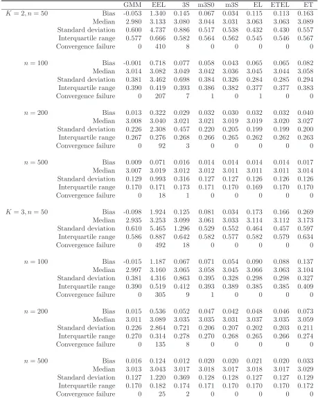
Table 1 displays the simulated median, bias, standard deviations, interquartile range and the

(24)

large number of convergence failure for the EEL estimator in particular in small samples and also with

increasing number of moment restrictions. This does not come as a surprise since the continuously

updated GMM of Hansen, Heaton and Yaron (1996) is also known to potentially display several outliers

and this estimator is known to be identical to the EEL estimator. The 3S estimator also displays

some outliers but much more rarely than the EEL estimator. Note that the number of outliers here

increases with smaller sample size and larger number of moment restrictions. We explain the failure

of the EEL and the 3S by the fact that the implied probabilities are not internally guaranteed to

be non negative. This leads to poor estimates of the Jacobian and the variance of the estimating

function and translates into some instability of both estimators. None of the other estimators shows

any systematic case of convergence failure. In that respect and by comparing the 3S estimator to the

m3S0 and m3S estimators we can conclude that the shrinkage of the implied probabilities helps to

increase the computation efficiency of the 3S estimator.

The outliers displayed by the EEL and the 3S estimators make them less efficient and often much

more biased than the other estimators. The m3S0, m3S, EL and ETEL estimators tend to have the

same bias in moderate size samples. The similarity of the simulated bias of the m3S and EL estimators

is a confirmation of our theory. The m3S0 and the m3S estimators even appear to have a smaller bias

for n= 50 and 100 in this design with the m3S outperforming, in general, the m3S0. It is also clear

that the GMM and the ET estimators do not share the same higher order bias as the other estimators

since, even for n= 500, their simulated biases are significantly different. This confirms the theory of

Newey and Smith (2004) namely that the GMM and the ET estimators have sources of higher order

bias different from the EL estimator.

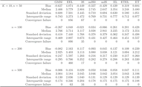
This Monte Carlo experiment does not show a clear evidence of the “no-moment” problem as

outlined by Guggenberger (2008). The large standard deviations of the 3S and EEL estimators in

small samples are down to outliers and seem to match the other estimators’ standard deviations as

the sample size grows. These outliers result from computation issues and their inflating effect on the

standard deviations is confirmed by the interquartile ranges which are of similar magnitude across all

the considered estimators.

Finally, all of these estimators seem sensitive to the number of moment conditions as they display

a larger amount of bias with increasing model size.

√_n

-convergence and Gaussianity under misspecification

We illustrate the behaviour of the three-step estimators under global misspecification using Designs C

(25)

by inner-outer loops optimizations. The true and pseudo-true parameter values being 0, we consider

the interval [−22.5,22.5] as the parameter set for the estimation purpose. We consider as convergence

failure the occurrence of corner solutions or the cases where either the inner or the outer loop

opti-mization routine fails. The simulated statistics in Table 2 are calculated without the failed samples.

The first-step GMM estimator is calculated with the weighting matrixW = (u_|v) with u= (1,0)′ and

v= (0,2/3)′. W is so chosen to reduce the weight on higher moments in the GMM objective function.

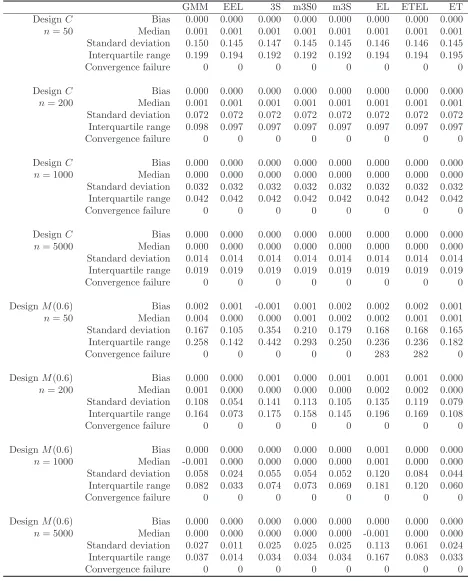
As reported by Table 2, the EL and ETEL estimators fail to converge in 2.83% of the simulated

samples for the design M(0.6) with n = 50 and in 0.01% of the simulated samples for the design

M(0.8) also withn= 50. The failure of the ETEL is clearly related to the failure of its EL step. This

shortcoming highlights some critical issue with the computation of EL in misspecified models.

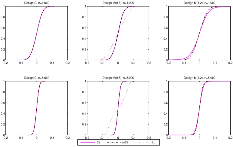
Table 2 displays the simulated standard errors for all of the estimators. In the correctly specified

model, the simulated standard errors are the same for all of the estimators. This, once again, confirms

that these estimators have the same asymptotic distribution as predicted by the theory. The cumulative

distribution functions plotted by Figure 2 also confirm this theoretical result.

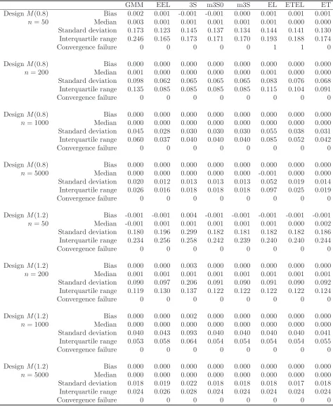
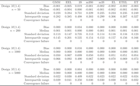
For the misspecified models, from our theory, we expect the simulated standard deviations of the

3S and m3S estimators to shrink by approximately 2 from n= 50 to n= 200 and by approximately

√

5 from n= 1,000 to n= 5,000. From the standard deviations displayed by Table 2 for M(s), s=

0.6,0.8,1.2,1.4, the 3S and m3S estimators have their standard deviations shrinking by approximately

2 from n = 50 to n = 200 and √5 from n = 200 to n = 1,000 and n = 1,000 to n = 5,000 as

expected. This is a confirmation of our theory. Even though we do not study the behaviour of the

EEL estimator in misspecified models, our simulation results suggest that this estimator may stay

√

n-convergent in misspecified models. The same observation is valid for the m3S0 estimator though

no asymptotic theory is available for this estimator in the case of global misspecification and its

asymptotic distribution robust to global misspecification is not known. The √n-convergence of the

GMM estimator in this experiment confirms the results of Hall and Inoue (2003).

The results for ET and ETEL estimators confirm the related literature. Their simulated standard

deviations seem to shrink by pn2/n1 as the sample size grows from n1 to n2. However, it appears

that the design M(0.6) sees the standard deviation of ETEL decrease by a narrower proportion than

expected from n = 1,000 to n = 5,000. This is likely related to some impact of EL which is the

poorest for this design.

The result of Schennach (2007) regarding the EL estimator in globally misspecified models is

confirmed by the designs M(0.6) and M(0.8). The simulated standard deviation of this estimator

(26)

2, one can also notice some distortion of the EL estimator as the sample size grows in misspecified

models. It is however worthwhile to mention that the EL behaves seemingly as a √n-convergent

estimator in the misspecified designsM(1.2) andM(1.4).

5 Conclusion

The three-step Euclidean likelihood estimator and its corrected version as proposed by Antoine, Bonnal

and Renault (2007) are computationally appealing and also higher order equivalent to the empirical

likelihood estimator in well specified models as their difference is Op(n−3/2).

This paper studies the 3S and the corrected 3S estimators under global misspecification and shows

that the 3S estimator remains √n-convergent in misspecified models and its asymptotic distribution

robust to global misspecification is derived. As for the corrected 3S estimator, it appears more difficult

to analyze in global misspecification context because of the lack of smoothness in the shrinkage factor.

We propose a slight modification of the shrinkage factor allowing to control its growing rate as it

diverges in the case of global misspecification. We label the resulting estimator themodified three-step Euclidean likelihood (m3S) estimator. We show that the m3S estimator is also higher order equivalent

to the EL estimator in well specified models while staying√n-convergent and asymptotically Gaussian

in globally misspecified models. Its asymptotic distribution robust to misspecification is also proposed.

These properties make the 3S and the m3S estimators very attractive alternative to the exponentially

tilted empirical likelihood (ETEL) estimator proposed by Schennach (2007) since they have the same

enjoyable properties of this latter in addition to being computationally more convenient.

There are some lines of extension of this work that we plan for future research. The empirical

likelihood ratio parameter and specification tests as proposed by Owen (1990) and Qin and Lawless

(1994) are known to outperform their existing alternative such as the Hansen’s (1982) GMM

overi-dentification test. However, these tests are computationally demanding as they depend on the full

derivation of the EL estimator. It could be of some interest to study the properties of these tests when

the three-step and modified three-step Euclidean likelihood estimators are used instead of the EL estimator. A higher order equivalence between the new tests and their original versions may suggest

(27)

[image:27.612.118.507.99.349.2]

Figure 1: Simulated cumulative distribution function of the 3S, m3S and EL estimators. Design D.

2 2.5 3 3.5 4 4.5 0 0.2 0.4 0.6 0.8 1 K=2, n=200

2 2.5 3 3.5 4 4.5 0 0.2 0.4 0.6 0.8 1 K=2, n=500

2 2.5 3 3.5 4 4.5 0 0.2 0.4 0.6 0.8 1 K=3, n=200

2 2.5 3 3.5 4 4.5 0 0.2 0.4 0.6 0.8 1 K=3, n=500

3S m3S EL

2 2.5 3 3.5 4 4.5 0 0.2 0.4 0.6 0.8 1 K=10, n=200

2 2.5 3 3.5 4 4.5 0 0.2 0.4 0.6 0.8 1 K=10, n=500

Figure 2: Simulated cumulative distribution function of the 3S, m3S and EL estimators. Well specified vs misspecified models. Designs C and M

−0.20 −0.1 0 0.1 0.2 0.2

0.4 0.6 0.8 1

Design C, n=1,000

−0.20 −0.1 0 0.1 0.2 0.2

0.4 0.6 0.8 1

Design C, n=5,000

−0.20 −0.1 0 0.1 0.2 0.2

0.4 0.6 0.8 1

Design M(0.8), n=1,000

−0.20 −0.1 0 0.1 0.2 0.2

0.4 0.6 0.8 1

Design M(0.8), n=5,000

3S m3S EL

−0.20 −0.1 0 0.1 0.2 0.2

0.4 0.6 0.8 1

Design M(1.2), n=1,000

−0.20 −0.1 0 0.1 0.2 0.2

0.4 0.6 0.8 1

[image:27.612.118.506.435.681.2]

(28)

[image:28.612.76.535.99.674.2]

Table 1: The simulated bias, median, standard deviation, and interquartile range of the GMM, EEL, 3S, m3S0, m3S, EL, ETEL and ET estimators from Design D

GMM EEL 3S m3S0 m3S EL ETEL ET

K= 2, n= 50 Bias -0.053 1.340 0.145 0.067 0.034 0.115 0.113 0.163 Median 2.980 3.133 3.080 3.044 3.031 3.063 3.063 3.089 Standard deviation 0.600 4.737 0.886 0.517 0.538 0.432 0.430 0.557 Interquartile range 0.577 0.666 0.582 0.564 0.562 0.545 0.546 0.567

Convergence failure 0 410 8 0 0 0 0 0

n= 100 Bias -0.001 0.718 0.077 0.058 0.043 0.065 0.065 0.082 Median 3.014 3.082 3.049 3.042 3.036 3.045 3.044 3.058 Standard deviation 0.381 3.462 0.698 0.384 0.326 0.284 0.285 0.294 Interquartile range 0.390 0.419 0.393 0.386 0.382 0.377 0.377 0.383

n= 200 Bias 0.013 0.322 0.029 0.032 0.030 0.032 0.032 0.040 Median 3.008 3.040 3.021 3.021 3.019 3.019 3.020 3.027 Standard deviation 0.226 2.308 0.457 0.220 0.205 0.199 0.199 0.200 Interquartile range 0.267 0.276 0.268 0.266 0.265 0.262 0.262 0.263

K= 3, n= 50 Bias -0.098 1.924 0.125 0.081 0.034 0.173 0.166 0.269 Median 2.935 3.253 3.099 3.061 3.033 3.114 3.112 3.173 Standard deviation 0.610 5.465 1.296 0.529 0.552 0.464 0.457 0.597 Interquartile range 0.586 0.887 0.642 0.582 0.577 0.582 0.579 0.634

(29)

Table 1 (Continued): The simulated bias, median, standard deviation, and interquartile range of the GMM, EEL, 3S, m3S0, m3S, EL, ETEL and ET estimators from Design D

K= 10, n= 50 Bias -0.627 4.074 -0.449 -0.327 -0.429 0.439 0.319 0.684 Median 2.466 3.779 2.804 2.745 2.647 3.354 3.248 3.480 Standard deviation 0.688 7.501 2.445 0.710 0.694 0.630 0.580 1.051 Interquartile range 0.783 3.273 1.472 0.769 0.731 0.777 0.712 0.977

n= 100 Bias -0.267 4.048 -0.021 0.034 -0.066 0.261 0.201 0.428 Median 2.766 3.714 3.117 3.038 2.941 3.225 3.172 3.354 Standard deviation 0.418 7.440 1.768 0.378 0.379 0.362 0.347 0.498 Interquartile range 0.469 2.007 0.673 0.431 0.427 0.463 0.451 0.557

[image:29.612.70.544.99.390.2]

(30)

[image:30.612.70.538.99.680.2]

Table 2: The simulated bias, median, standard deviation, and interquartile range of the GMM, EEL, 3S, m3S0, m3S, EL, ETEL and ET estimators for Designs C and M

DesignC Bias 0.000 0.000 0.000 0.000 0.000 0.000 0.000 0.000

n= 50 Median 0.001 0.001 0.001 0.001 0.001 0.001 0.001 0.001 Standard deviation 0.150 0.145 0.147 0.145 0.145 0.146 0.146 0.145 Interquartile range 0.199 0.194 0.192 0.192 0.192 0.194 0.194 0.195

DesignC Bias 0.000 0.000 0.000 0.000 0.000 0.000 0.000 0.000

DesignM(0.6) Bias 0.002 0.001 -0.001 0.001 0.002 0.002 0.002 0.001

DesignM(0.6) Bias 0.000 0.000 0.001 0.000 0.001 0.001 0.001 0.000

DesignM(0.6) Bias 0.000 0.000 0.000 0.000 0.000 0.001 0.000 0.000

n= 1000 Median -0.001 0.000 0.000 0.000 0.000 0.001 0.000 0.000 Standard deviation 0.058 0.024 0.055 0.054 0.052 0.120 0.084 0.044 Interquartile range 0.082 0.033 0.074 0.073 0.069 0.181 0.120 0.060

DesignM(0.6) Bias 0.000 0.000 0.000 0.000 0.000 0.000 0.000 0.000

n= 5000 Median 0.000 0.000 0.000 0.000 0.000 -0.001 0.000 0.000 Standard deviation 0.027 0.011 0.025 0.025 0.025 0.113 0.061 0.024 Interquartile range 0.037 0.014 0.034 0.034 0.034 0.167 0.083 0.033