Munich Personal RePEc Archive
Accounting for Incomplete Pass-Through
Nakamura, Emi and Zerom, Dawit
November 2008
Online at
https://mpra.ub.uni-muenchen.de/14389/
Accounting for Incomplete Pass-Through
Emi Nakamura Columbia University
Dawit Zerom
California State University, Fullerton∗
November 2008
Abstract
Recent theoretical work has suggested a number of potentially important factors in causing incomplete pass-through of exchange rates to prices, including markup adjustment, local costs and barriers to price adjustment. We empirically analyze the determinants of incomplete pass-through in the coffee industry. The observed pass-pass-through in this industry replicates key features of pass-through documented in aggregate data: prices respond sluggishly and incompletely to changes in costs. We use microdata on sales and prices to uncover the role of markup adjustment, local costs, and barriers to price adjustment in determining incomplete pass-through using a structural oligopoly model that nests all three potential factors. The implied pricing model explains the main dynamic features of short and long-run pass-through. Local costs reduce long-run pass-through by a factor of 59% relative to a CES benchmark. Markup adjustment reduces pass-through by an additional factor of 33%, where the extent of markup adjustment depends on the estimated “super-elasticity” of demand. The estimated menu costs are small (0.23% of revenue) and have a negligible effect on long-run pass-through, but are quantitatively successful in explaining the delayed response of prices to costs. We find that delayed pass-through in the coffee industry occurs almost entirely at the wholesale rather than the retail level.
Keywords: exchange rate pass-through, menu costs, discrete choice model. JEL Classifications: F10, L11, L16.
1
Introduction
A substantial body of empirical work documents that exchange rate pass-through to prices is delayed and incomplete (Engel, 1999; Parsley and Wei, 2001; Goldberg and Campa, 2006). These studies show that the prices of tradable goods respond sluggishly and incompletely to variations in the nominal exchange rate. An increase in the exchange rate leads to a substantially less than proportional increase in traded goods prices; and much of the price response occurs with a substantial delay.1
Recent theoretical work has suggested a number of potentially important factors in explaining incomplete pass-through. First, in oligopolistic markets, the response of prices to changes in costs depends both on the curvature of demand and the market structure (Dornbusch, 1987; Knetter, 1989; Bergin and Feenstra, 2001). Second, local costs may play an important role in determining pass-through (Sanyal and Jones, 1982; Burstein, Neves and Rebelo, 2003; Corsetti and Dedola, 2004). Local costs drive a wedge between prices and imported costs that is unresponsive to exchange rate fluctuations. As a consequence, if local costs are large, even a substantial increase in the price of an imported factor of production could have little impact on marginal costs. Third, price rigidity and other dynamic factors have the potential to contribute to incomplete pass-through (Giovannini, 1988; Kasa, 1992; Devereux and Engel, 2002; Bacchetta and van Wincoop, 2003).
We study pass-through in the coffee industry. Coffee is the world’s second most traded commod-ity after oil. Over the past decade, coffee commodcommod-ity prices have exhibited a remarkable amount of volatility. However, retail and wholesale coffee prices have responded sluggishly and incompletely to changes in imported commodity costs—an important feature of the aggregate evidence.2
The response of prices to changes in costs is intimately related to the response of prices to exchange rates. Indeed, the equations used to estimate the response of prices to exchange rates are derived from equations that relate prices to marginal costs. In standard exchange rate pass-through regressions, foreign inflation is used to proxy for marginal costs, and prices are regressed separately on costs and exchange rates. The coffee market is an ideal laboratory to study how costs pass-through into prices since a large fraction of marginal costs are observable for this industry. Coffee commodity costs are, moreover, buffeted by large, observable, non-monetary factors. This makes price responses easier to interpret than in the standard case of exchange rate pass-through, since exchange rate movements may be closely linked to monetary factors, at least in the long run, and such factors may have a direct effect on prices, independent of movements in the exchange rate (Corsetti, Dedola and Leduc, 2008; Bouakez and Rebei, 2008).3
For both retail and wholesale prices, a one percent increase in coffee commodity costs leads to an increase in prices of approximately a third of a percent over the subsequent 6 quarters (we refer to this as long-run pass-through). More than half of the price adjustment occurs with a delay of one quarter or more. By wholesale prices, we mean the prices charged by coffee roasters like Folgers and Maxwell House, which we also refer to as manufacturer prices.
1
See also Frankel, Parsley, and Wei (2005) and Parsley and Popper (2006).
2
This has generated considerable public interest in coffee markets. In 1955, 1977 and 1987, the US Congress launched inquiries into the pricing practices of coffee manufacturers.
3
Reduced form regressions indicate that delayed pass-through in this industry occurs almost entirely at the wholesale level. This evidence suggests that, to the extent that barriers to price adjustment contribute to delayed pass-through in this industry, it is wholesale price rigidity that matters. Recent research on price dynamics has focused on price rigidity at the retail level, partly because retail price data are more readily available to researchers. The finding that, at least in the coffee industry, the majority of incomplete pass-through arises at the level of wholesale prices indicates that studies that focus exclusively on retail prices may be incomplete in an important way.4 We document substantial rigidity in coffee prices at both the wholesale and retail level: over
the time period we consider, manufacturer prices of ground coffee adjust on average 1.3 times per year, while retail prices excluding sales adjust on average 1.5 times per year over the same time period. The frequency of wholesale price adjustment is highly correlated with commodity cost volatility: wholesale prices adjust substantially more frequently during periods of high commodity cost volatility. Goldberg and Hellerstein (2007) similarly document an important role for wholesale price rigidity in the beer market using data from a large US supermarket chain.
We build a structural model of the coffee industry and investigate its success in explaining the facts about pass-through. We begin by estimating a model of demand for coffee. The coffee market, like most markets, is best described as a differentiated products market. The main difficulty of estimating demand curves in a differentiated products industry is that an unrestricted specification of the dependence of aggregate demand on prices leads to an extremely large number of free parameters. It is therefore useful to put some structure on the nature of demand. We do this by specifying a discrete choice model of demand (McFadden, 1974). This type of structural model places restrictions on the cross-price elasticities by assuming utility maximizing behavior, thereby resulting in a substantially more parsimonious model. We follow Berry, Levinsohn, and Pakes (1995) in estimating a random coefficients model with unobserved product characteristics. An advantage of the coffee industry in estimating the demand system is that coffee prices are buffeted by large exogenous shocks to supply in the form of weather shocks to coffee producing countries. We use these weather shocks as instruments to identify the price elasticity of demand.
We combine this demand model with a structural model of the supply side of the coffee industry. We fix the number of firms and the products produced by the firms to match the observed industry structure. We account for the observed degree of price rigidity by assuming that firms must pay a “menu cost” in order to adjust their prices. According to this model, firms face a fixed cost of price adjustment that leads them to adjust their prices infrequently: we do not take a stand on the sources of the barriers to price adjustment.5 The barriers to price adjustment imply that the model is a dynamic game. We then analyze the equilibrium response of prices to costs in a Markov perfect equilibrium of this model. In our baseline estimation procedure, we use local costs estimated from
4
Retailers nevertheless play an important role in determining the level of pass-through since they insert an ad-ditional wedge between imported costs and prices. Furthermore, though we do not analyze this channel, retailer-manufacturer interactions may play an important role in determining retailer-manufacturer pricing behavior, and may even be one motive for manufacturer-level price rigidity. The role of retail behavior in determining pricing behavior is analyzed in detail by Hellerstein (2005) and Villas-Boas (2007).
5
a static model in order to avoid the problem of searching over a large number of parameters in the dynamic estimation procedure. We also consider an alternative procedure in which we estimate a common component in marginal costs as part of the dynamic estimation procedure. Incorporating price rigidity in the model is crucial both because of its impact on short-run dynamics and because ignoring these factors could otherwise bias our estimates of the role of local costs and markup adjustment (Engel, 2002).
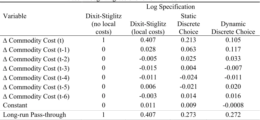
We find that the dynamic pricing model, estimated using panel data on prices and market shares, replicates the main dynamic features of pass-through in the short and long-run. We use the model to determine the role of local costs, markup adjustment and menu costs in long-run pass-through. We do this by comparing our baseline dynamic model to successively simpler models. We find that local costs reduce pass-through by a factor of 59% relative to a CES benchmark, while markup adjustment reduces pass-through by an additional factor of 33%. Menu costs have a negligible effect on long-run pass-through, though they play an important role in explaining short-run pricing dynamics as we discuss above.6 Our conclusions underscore the need to allow for additional channels
of incomplete pass-through in the large literature in international macroeconomics in which rigid prices are the main source of imperfect adjustment of prices to costs.7
In comparing the model to the data, we emphasize three main features of our results. First, in the long-run, markup adjustment in response to cost shocks is substantial: firms are estimated to compress their gross margins on average by a factor of 1/3 in response to a marginal cost increase. This implies that a one percent increase in coffee commodity costs leads to a “long-run” pass-through into prices of approximately a third of a percent over the subsequent 6 quarters, despite a much larger fraction of marginal costs being accounted for by green bean coffee. Klenow and Willis (2006) coin the term “super-elasticity” of demand for the percentage change in the price elasticity for a given percentage increase in prices and show that it is a key determinant of how prices respond to costs in macroeconomic models. While the Dixit-Stiglitz model implies a super-elasticity of demand of 0, we estimate a median super-super-elasticity of demand of 4.64, generating a substantial motive for markup adjustment.8
Second, the menu cost model parameterized to fit the overall frequency of price change is quantitatively successful in matching the short-run dynamics of pass-through. Most of the price adjustment occurs in the quarters after the initial change in costs. The menu costs imply a sub-stantial amount of price rigidity: prices adjust only every 9 or 10 months. Yet, menu costs are found to play a negligible role in explaining long-run pass-through after 6 quarters.
Third, our analysis strongly favors the dynamic menu cost model over a pricing model in which firms set prices purely according to a fixed schedule as in the Taylor model (Taylor, 1980) or change prices with a fixed probability as in the Calvo model (Calvo, 1983). The central prediction of the menu cost model is that price adjustments occur more frequently in periods when marginal costs change substantially. While this is an important prediction of the menu cost model, it has been
6
These results echo the findings of Goldberg and Verboven (2001) for the European car market, as well as the findings of Burstein, Eichenbaum, and Rebelo (2005) for the behavior of tradable goods prices following large deval-uations in terms of the large role played by local costs. Our findings are also consistent with the results of Lubik and Schorfheide (2005). For other interesting attempts to distinguish between markup adjustment and price rigidity in explaining exchange rate pass-through see Giovannini (1988) and Marston (1990).
7
See e.g. Engel (2002) for a discussion of this literature.
8
difficult to study given the difficulty of observing marginal costs. This prediction of the model is borne out strongly by the data. There is a strong positive relationship between turbulence in the coffee commodity market and the frequency of price change in a given year.9 Moreover, the
observed price rigidity and delayed response of prices to costs can be explained by a plausibly small magnitude of adjustment costs (0.23% of revenue). Small menu costs are found to generate a large amount of price rigidity both because of relatively inelastic demand and because local costs account for a large fraction of marginal costs.
It is worth emphasizing that neither the model’s fit to the dynamics of pass-through nor its fit to the timing of price adjustments are “guaranteed” by the estimation procedure: the estimation procedure uses information on long-run average prices, demand, and frequency of price change, but does not make use of the empirical evidence on pass-through or the timing of price adjustments.
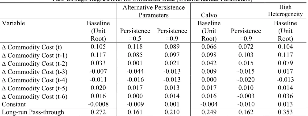
The predictions of this type of model depend on a number of factors that do not arise in a static context. Since firms consider not only current but future costs in making pricing decisions, pass-through depends on the dynamics of marginal costs. In the case of a monopolistic competition model with a symmetric profit function, it is clear by symmetry that if marginal costs have a unit root then prices adjust to the static optimum conditional on adjusting (Dixit, 1991). This intuition essentially goes through in the present model as well—implying that menu costs have little impact on long-run pass-through in the unit root case. The unit root case is relevant for the coffee market since we cannot reject the hypothesis that coffee commodity costs have a unit root. Yet, we show that even in the unit root case, dynamic considerations matter for the magnitude of the menu costs required to explain a given amount of price rigidity. We also investigate quantitatively how sensitive our results on both pass-through and the magnitude of the menu cost are to the persistence of costs, the degree of consumer heterogeneity and the model of price adjustment behavior (i.e. menu cost vs. the Calvo (1983) model).
The basic approach we use to study pass-through in this industry builds on recent work by Goldberg and Verboven (2001) and Hellerstein (2005). These papers provide detailed models of pricing in particular industries, and analyze their models’ implications for pass-through. In partic-ular, Hellerstein (2005) introduces a novel decomposition of the sources of incomplete pass-through into non-traded costs and markup adjustment. These analyses have focused on the contemporane-ous response of prices to changes in costs. Yet, the delayed response of prices to costs suggests that dynamic factors are also important in explaining pass-through and may affect existing empirical results. Engel (2002) argues that Goldberg and Verboven (2001) overestimate the role of local costs because they do not allow for price rigidity.
This paper extends the existing static models to incorporate additional empirical facts about delayed and incomplete pass-through. Goldberg and Hellerstein (2007) carry out a closely related study of the role of price rigidity in pass-through in the beer market, but approximate the firms’ pricing policies using a static model. In contrast, we firm pricing policies in a dynamic framework. The menu cost pricing model in this paper builds on Slade (1998, 1999) and Aguirregabiria (1999) who incorporate menu costs into industrial organization models of price adjustment in order to estimate the barriers to price adjustment. Another closely related paper is Kano (2006) which also solves for the Markov Perfect Equilibrium of a dynamic menu cost model using numerical
9
methods. More broadly, this paper is related to a large empirical literature on cost pass-through as well as a growling literature on state-dependent pricing models solved using numerical methods.10 Bettendorf and Verboven (2000) study the relationship between Dutch coffee prices and commodity costs in a static oligopoly model and find similar results on the magnitude of non-coffee bean costs. One issue that arises in this type of analysis based on a particular industry is the extent to which conclusions based on one particular industry can be extended to understand pricing dynamics in other industries. The major players in this industry—Proctor & Gamble, Kraft and Sara Lee—are some of the world’s largest consumer packaged goods companies, suggesting that studying their pricing behavior in one market may give insights into their behavior in other markets as well. The extent of price rigidity observed in the coffee industry is also typical: the average duration of wholesale prices is approximately 9 months, which is similar to the median duration of prices in the U.S. producer price index (Nakamura and Steinsson, 2008). Our conclusions about the importance of price dynamics at the retail versus the wholesale level may also be useful in understanding price dynamics in other industries. Retailers play an important role in numerous sectors of the economy, particularly food, clothing and household furnishings, which account for more than 30% of US consumption. Understanding the relationship between retail and wholesale prices is therefore crucial in understanding price dynamics for a large part of the US economy. Relative to other industries, imported costs may be a particularly large fraction of marginal costs in the coffee industry—indeed, we selected the coffee industry in part because of the disproportionate share of marginal costs accounted for by imported intermediate goods (coffee beans).11 Regarding our
conclusions about the role of markup adjustment in explaining long-run pass-through, since coffee costs are highly correlated across firms, different coffee producers’ incentives to adjust their prices tend to be coordinated. In markets where firms face disparate cost shocks, the incentive for a firm to compress its markup in response to a cost increase may be even greater. Finally, our conclusions regarding the limited role of menu costs in explaining long-run pass-through after 6 quarters depend importantly on the persistence and volatility of commodity costs, but are relevant to pass-through of other highly persistent costs such as exchange rates and wages. Our conclusions regarding the role of menu costs also depend on the nature of strategic interactions implied by our estimated model of demand, as we discuss in section 7.
The paper proceeds as follows. Section 2 provides an overview of the data used in the paper. Section 3 presents stylized facts about price adjustment in the coffee industry. Section 4 describes the demand model and presents empirical estimates of the demand side of the model. Section 5 presents estimates of local costs derived using a static oligopoly model. We evaluate the robustness of these estimates to dynamic considerations in appendix B. Section 6 presents the full supply side of the model. This section presents the menu cost oligopoly model, as well as our menu cost estimates based on the dynamic model. Section 7 establishes the predictions of the model for incomplete pass-through in the short and long-run, and investigates the relative importance of markup adjustment, local costs and menu costs. Section 8 contains a number of counterfactual
10
In the cost pass-through literature, see Kadiyali (1997), Gron and Swenson (2000) and Levy et al. (2002). See also Bettendorf and Verboven (2000) and the references therein for specific analyses of coffee prices in various countries. A recent example of a numerical state dependent pricing model in the international economics literature is Floden and Wilander (2004). See also Gross and Schmitt (2000) for an alternative explanation of delayed pass-through.
11
simulations that investigate how our estimates of menu costs and results on incomplete pass-through depend on the persistence of costs, the curvature of demand and the model of price adjustment behavior. Section 9 concludes.
2
Data on Prices and Costs
We pull together data on prices and costs from a number of sources to develop our model of the coffee industry. We use data on prices and sales from two industry sources. Our source for retail price and sales data is monthly AC Nielsen data. These data are market-level average prices and sales for the period 2000-2004. We use these data to construct series on retail prices and market shares.12
We use wholesale price data from PromoData. Promodata collects data on manufacturer prices for packaged foods from grocery wholesalers. Promodata collects its information from the largest grocery wholesaler in a given market but does not identify the wholesaler for confidentiality reasons. These data provide the price per case charged by the manufacturer to the wholesaler for a particular UPC in a particular week. The data start in January 1997 and end in December 2005. Because Promodata surveys a much less complete array of markets and wholesalers than AC Nielsen, the wholesale price data cover a substantially less complete array of markets than the retail data. Data are available for 31 of the 50 retail markets, though the time span covered varies by market, leading to an unbalanced panel of observations. Moreover, data are typically only available for the leading products in each market. The wholesale price data have certain advantages over the retail data. In particular, since the wholesale data are prices for individual products from particular manufacturers to a particular wholesaler in a particular week, we can use these data to analyze price rigidity.
In a recent report by the Brazil Information Center (Brazil-Information-Center-Inc., 2002), about half of 20 large US retailers interviewed reported using grocery wholesalers, though the fraction was lower among the largest supermarkets in this group. In general, the price quoted to a grocery wholesaler is non-negotiable, and the product is delivered directly to the wholesaler’s warehouse. The grocery wholesaler then resells the product to a supermarket.
The wholesale price data contain information on both base prices and “trade deals”. Trade deals are discounts offered to the grocery wholesalers to encourage promotions. For some types of trade deals, manufacturers require proof that a promotion has been carried out in order to redeem the discount. According to a former grocery wholesale executive, since advertising is often carried out collectively by grocery stores associated with a particular wholesaler, in many cases, the funds associated with the trade deal are used by a grocery collective for promotional purposes rather than being passed on to individual stores. The cost pass-through regressions we present are for prices including trade deals, though our results on pass-through are similar both including and excluding trade deals.
The commodity price data are based on commodity prices on the New York Physicals market collected by the International Coffee Organization (ICO). We focus on price responses to a “com-posite commodity index” that we construct in the following way. We take a weighted average of the
12
commodity prices for Colombian Mild Arabicas, Other Mild Arabicas, Brazilian and Other Natural Arabicas, and Robustas. We weight the commodity prices for the different varieties based on the average composition of U.S. coffee consumption from Lewin, Giovannucci, and Varangis (2004) over the years 1993-2002. These weights have remained relatively stable over the sample period. We adjust the commodity price for the fact that roasted green coffee beans lose about 19% of their weight during the roasting process.
To construct the graphs of aggregate series in section 3, we make use of retail and wholesale price indexes from the Bureau of Labor Statistics. In particular, we make use of the “ground coffee” retail price index and the “roasted coffee” wholesale price index downloaded from the Bureau of Labor Statistics webpage.
In principle, it would be preferable to separately analyze the response of coffee retail and wholesale prices to movements in the prices of different types of green bean coffee.13 Unfortunately,
reliable estimates of the composition of different brands of coffee by coffee bean type are not available. However, the effect of analyzing responses to the coffee commodity index rather than individual coffee types is likely to be small for two reasons. First, the prices for different types of green bean coffee covary strongly. Second, as we note above, the consumption weights of the different types of coffee for the U.S. as a whole have changed little over the sample period.
3
Cost Pass-Through Regressions
Let us begin by looking at the relative movements of coffee prices and costs over the past decade.14
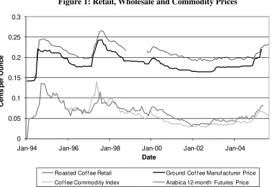
Figure 1 presents a graph of average retail, wholesale and commodity prices in US dollars per ounce. To be clear about terminology, we shall refer to the price charged by supermarkets to consumers as theretail price, the price charged by coffee roasters such as Folgers and Maxwell House to grocery wholesalers as the wholesale price, and the price of green bean coffee on the New York market as thecommodity cost.
The vast majority of coffee sold in the U.S. is imported in the form of green bean coffee (the largest coffee producing countries are Brazil, Colombia and Vietnam). Coffee manufacturers roast, grind, package and deliver the coffee to the American market.15 Green bean coffee prices were highly volatile over the period we study, losing almost two thirds of their value between 1997 and 2002. Most of the volatility in commodity costs arises from weather conditions in coffee producing countries, planting cycles and new players in the coffee market. Since coffee commodity prices are quoted in U.S. dollars, commodity prices have also been affected by the rise and fall of the value of the U.S. dollar.
We document three facts about prices and costs in the coffee market: 1)the pass-through of coffee commodity prices to retail and wholesale coffee prices, 2)the response of retail to wholesale coffee prices, and 3)the extent of price rigidity in wholesale prices in the coffee industry. First, we document the dynamics of the relationship between prices and costs. Figure 1 shows that retail and
13
In some industries, shifting input composition plays an important role in determining cost pass-through. See Gron and Swenson (2000).
14
This section draws heavily on the analysis in Leibtag et al. (2005).
15
wholesale prices tracked commodity prices closely over this period. The close relationship between prices and commodity costs is not surprising given the large role of green bean coffee in ground coffee production. Industry estimates suggest that green bean coffee accounts for more than half of the marginal costs of coffee production.16 To quantify this relationship, we estimate the following
standard pass-through regression,
∆ logpljmt=a+
6
X
k=1
bk∆ logCt−k+
4
X
k=1
dkqk+ǫ, (1)
wherel=r, w, ∆ logpr
jmt is the log retail price change of product j in marketm, ∆ logpwjmt is the
corresponding log wholesale price change, ∆ logCt−kis the log commodity cost index,qtis a quarter
of the year dummy, a, bk and dk are parameters and ǫ is a mean zero error term. The wholesale
price series include trade deals; the results excluding trade deals are virtua.17 The coefficientsb
k
may be interpreted as the percentage change in prices associated with a given percentage change in commodity costs k quarters ago. The empirical model follows the approach of Goldberg and Campa (2006). The model is motivated by the fact that, as in Goldberg and Campa (2006), the regressor is highly persistent: a Dickey-Fuller test for the hypothesis of a unit root in commodity prices cannot be rejected at a 5% significance level. Goldberg and Campa (2006) define the long-run rate of pass-through in this model as the sum of the coefficients P6
k=1bk. We selected the number
of lags included in the regression such that adding additional lags does not change the estimated long-run rate of pass-through. We estimate the model using the retail and wholesale price data described in Section 2, for quarterly changes in prices and costs over the 2000-2005 period.18
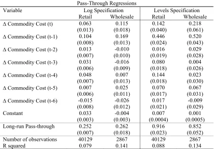
Table 1 presents the results of the pass-through regression for retail and wholesale prices. We present estimates from two types of pass-through regressions. Columns 1 and 2 of table 1 present the results of the standard pass-through regression (1). The results reflect a substantial amount of incomplete pass-through in percentage terms. The estimated long-run pass-through elasticity is 0.252 for retail prices and 0.262 for wholesale prices. In other words a one percent increase in commodity costs eventually leads to only about a quarter of a percent increase in coffee prices. We do not find evidence that prices systematically react asymmetrically to price increases or de-creases.19 This finding is consistent with the findings in Gomez and Koerner (2002) for the US, France and Germany. Table 1 also documents that there is a substantial delay in the response of prices to commodity costs. For both retail and wholesale prices, more than half of the adjustment to a change in costs occurs in the period after the cost shock.20 It is, of course, also possible to estimate standard exchange rate pass-through regressions instead of cost pass-through regressions.
16
For example, a major producer estimated in 1976 that green bean coffee accounted for 82% of marginal costs (Yip and Williams, 1985). Industry estimates suggest, however, that the fraction of marginal costs accounted for by commodity costs have since fallen with the price of green bean coffee.
17
Trade deals are slightly more common when commodity costs are low. The effect is, however, quantitatively small: an increase in green bean coffee costs by 1 cent lowers the frequency of trade deals by about 0.2 percentage points; the size of trade deals are not correlated in a statistically significant way with commodity costs.
18
The standard errors for all of the regressions in this section are clustered by unique product and market to allow for arbitrary serial correlation in the error term for a given product. See, for example, Wooldridge (2002) for a discussion of this procedure.
19
We considered asymmetries in the response of prices to commodity costs at 1-4 lags. See Leibtag et al. (2005) for a more detailed discussion of this issue.
20
Interestingly, these exchange-rate pass-through regressions yield substantially lower estimates of pass-through: 0.21 and 0.04 respectively, again with the majority of pass-through occurring after the initial quarter.
One might be concerned that long-term contracts for purchasing green bean coffee imply that the average purchasing price of coffee manufacturers may differ from the coffee commodity price. Yet, this concern ignores the fact that in an economic model, firms’ prices respond to marginal costs rather than accounting costs. While hedging contracts affect the firm’s total costs, they do not affect its marginal costs, so long as the firm is always on the margin of buying or selling at the observed commodity cost.
Columns 3 and 4 of table 1 present the results of the pass-through regression (1) in levels rather than logs. For this specification, the long-run pass-through of retail prices to commodity costs is 0.916, while the long-run pass-through to wholesale prices is 0.852. Thus, a one cent increase in commodity prices leads to slightly less than a one cent increase in prices.21 The difference
between the regressions in levels and logs is explained by the substantial wedge between observed prices and marginal costs, which implies that a one cent change corresponds to a substantially smaller percentage change in prices than costs.22 This alternative specification of the pass-through regression begs the question of whether it might be more relevant to consider cent-for-cent pass-through as a benchmark for “complete” pass-pass-through as opposed to a pass-pass-through elasticity of 1. Yet, a pass-through elasticity of 1 is an appealing benchmark both because it arises in the workhorse Dixit-Stiglitz model (absent local costs) and because it is only possible to calculate pass-through elasticities (rather than levels) using standard data sources on price indicies.23
Second, we document the responsiveness of retail prices to manufacturer prices. This analysis investigates to what extent delays in pass-through occur at the wholesale versus the retail level. This issue matters both for how we model price adjustment behavior, and what data are most relevant for parameterizing the model. In order to analyze this issue, we consider the following
21
An alternative approach would be to estimate a panel error correction model. We cannot reject the null of no cointegration of coffee prices and coffee bean costs in aggregate data over the time period we consider. Nevertheless, as a robustness check, we also estimated a number of specifications that allow for a cointegrating relationship between prices and green bean coffee costs. We estimated a vector error correction model (with a restricted constant) for aggregate data on ground coffee manufacturer prices and the commodity cost index (the data series underlying Figure 1) for the 1994-2005 period. This model implied similar results to specification 1: approximately cent-for-cent pass-through in the long-run with less than half of the pass-through occurring in the first quarter, though the parameter estimates were much less precise. Estimating panel vector error correction models for panel data remains econometrically challenging (Breitung and Pesaran, 2005) and a full analysis of these issues is beyond the scope of this paper. However, we also reestimated specification 1 in both levels and logs while including, as a vector error correction term, the price minus the commodity cost. These specifications yielded almost identical results to those reported in Table 1.
22
These statistics are for retail prices including temporary sales. A 1 cent per ounce increase in commodity costs is associated with a 0.03 cent decrease in the difference between base prices (excluding sales) and net prices (including sales)—about 3% of the overall pass-through, based on a fixed effects regression of the difference between base and net prices on commodity costs and quarter dummies. According to this metric, temporary sales contribute little to overall pass-through, though it is unclear how to interpret this fact given the complex dynamic response of demand to temporary sales.
23
regression of retail prices on wholesale prices,
∆prjmt=αr+
2
X
k=0
βkr∆pwjmt−k+
4
X
k=1
γrkqk+ǫ, (2)
where αr, βr
k and γkr are parameters, and ǫ is a mean zero error term. The wholesale price data
are likely to be a noisy proxy for the wholesale costs faced by any particular retailer. To avoid attenuation bias, we estimate this equation by instrumental variables regression with commodity costs as instruments.24 Table 2 reports the results of this regression. The estimated pass-through
coefficient on contemporaneous changes in wholesale prices is 0.958, with small and insignificant coefficients on the lagged wholesale price changes. This regression indicates that retail prices respond immediately and approximately cent-for-cent to changes in wholesale prices associated with cost shocks, indicating that almost all of the delays in pass-through in this market may be explained by delays at the wholesale level. This result motivates a focus on both documenting and explaining price adjustment at the wholesale level.
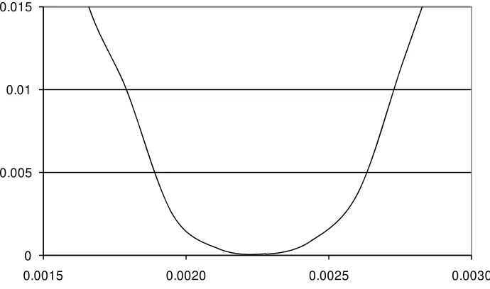
[image:12.612.204.411.97.133.2]Third, we document the extent of price rigidity in manufacturer prices in the coffee industry. Figure 2 presents a typical wholesale price series for coffee. The figure shows that wholesale coffee prices have sometimes remained unchanged for substantial periods of time. Since 1997, Proctor and Gamble (P&G), the maker of Folgers coffee has announced three major price increases and eight major price decreases.25 P&G commented to reporters in conjunction with its 2004 price
increase that P&G “increases product prices when it is apparent that commodity price increases will be sustained”. (Associated Press, Dec. 10 2004). Table 3 presents the statistics on the annual evolution of the frequency of price adjustment for wholesale and retail prices, where the frequency of price adjustment of retail prices is based on data from the consumer price index database analyzed in Nakamura and Steinsson (2008). The average frequency of wholesale price adjustment is 1.3 over the 1997-2005 period while the average frequency of retail price adjustment excluding retail sales is 1.5.26
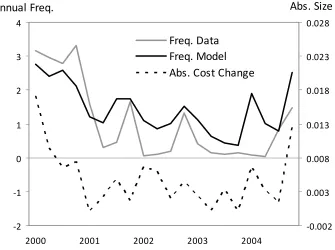
There is a strong and statistically significant relationship between commodity cost volatility and the frequency of price change. Table 4 presents statistics on the average number of wholesale price adjustments per year over the period 1997-2003. Over the years 1997 to 2005, the average number of price changes in a year varied between 0.2 and 4.3 for wholesale price changes not including trade deals. Figure 3 plots the relationship between the average frequency of wholesale price changes and the annual volatility of the monthly commodity cost index for the years 1997-2005, illustrating a strong positive relationship. These patterns reflect a large amount of synchronization in price-setting that coincides with times of high commodity cost volatility: in the quartile with the lowest
24
The instruments we use are current changes in the commodity cost index and 12 month Arabica futures prices as well as 6 lags of these variables.
25
These statistics are based on price change announcements reported in the Lexis Nexus news archive.
26
A key question in interpreting the evidence on wholesale price rigidity is whether rigid wholesale prices actually determine the retail prices faced by consumers. Since manufacturers and retailers interact repeatedly, the observed rigid prices may not be “allocative” (Barro, 1977). In particular, retail prices may react to cost shocks even when wholesale prices do not. We find little evidence of this phenomenon in the coffee market: conditional on wholesale prices, retail prices do not appear to react to changes in commodity prices. We estimated the regression, ∆ logpr
jmt=
η0
+P1
k=0η
C
k∆ logCt−k+P
1
k=0η
r k∆ logp
w jmt−k+
P4
k=1γ
r
kqk+ǫ, by instrumental variables regression with the same
instruments used to estimate equation (2). The current wholesale price pw
jmt had a coefficient of 1.001 while the
frequency of price change, less than 4.5% of products adjust their prices; while in the quartile with the highest frequency of price change, more than 65% of products adjust their prices.
4
Consumer Demand
The first building block of my structural model of the coffee industry is a model of consumer demand. We estimate a random coefficients discrete choice model for demand (Berry, Levinsohn and Pakes, 1995).27 In this model, the consumer is assumed to select the product that yields the
highest level of utility, where the indirect utility of individual i from purchasing product j takes the form,
Uijmt =α0i +α p
i(yi−prjmt) +xjβx+ξjmt+ǫijmt, (3)
whereαpi is the parameter governing the individual-specific marginal utility of income,yi is income,
pjmt is the price in market m at time t,xj is a vector of product characteristics,βx is a vector of
parameters, and ξjmt is an unobserved demand shifter that varies across products and regions.28
We also allow the consumer to select the outside option of not purchasing ground caffeinated coffee. Since the mean utility from the outside option is not separately identified, we normalize ξ0mt = 0
implying that the utility from the outside option is given byUi0mt=αipyi+ǫi0mt. For computational
tractability, the idiosyncratic error termǫijmtis assumed to be distributed according to the extreme
value distribution. Demand, in ounces of coffee, is then given by the market sharesjmt, the fraction
of consumers for whom product j yields the highest value of utility, multiplied by the size of the marketM.
The key advantage of this type of structural model relative to an unrestricted model of demand is that it allows for a substantial reduction in the number of parameters that must be estimated, while still allowing for a substantial amount of flexibility in substitution patterns. To build intuition, we begin by estimating the logit model, a simplified version of the full model in whichαpi =αp and
α0
i =α0 for alli. In this case, the model implies the following equation for aggregate shares,
logsjmt−logs0 =α0−αpprjmt+xjβ+ξjmt, (4)
whereα0is a constant. We estimate the model on monthly price and market share data for ground,
caffeinated coffee for 50 US markets as defined by AC Nielsen, where the prices and market shares are averages by market, brand, time period and size.29
To give a feel for the market structure of the coffee industry, let us note that some of the largest coffee manufacturers in the U.S. are Folgers and Maxwell House, which are owned by Proctor & Gamble and Kraft Foods respectively. The market for ground coffee is highly concentrated. Across markets, the median Herfindahl index is 0.34 and the median fraction of coffee sales accounted
27
Discrete choice models have been applied widely in the empirical organization literature. Other applications include shopping destination choice (McFadden, 1974), cereal (Nevo, 2001) and yogurt (Villas-Boas, 2004). See Anderson, Palma, and Thisse (1992) for an overview of this class of models.
28
This expression for indirect utility may be derived from a quasi-linear utility function. One way of interpreting this model is to view the consumer’s decision of what to consume as a discrete choice at each “consumption occasion”. Given micro-level data on consumers’ purchases, an alternative approach would be to estimate an explicit model of multiple discrete choices as in e.g. Hendel (1999).
29
for by Folgers and Maxwell house alone is 0.80. On average, each brand produces two sizes of ground caffeinated coffee, and three distinct coffee UPC’s. Among consumer packaged goods, “store brands” account for relatively small fraction of total sales (4.7%).
The model is estimated using the top 15 products by volume sold nationally over the 5 year sample period 2000-2004. These products account for 74% of the total AC Nielsen ground coffee sales over this period.30 To estimate the model, it is necessary to define the total potential market M. We define the relevant market as two cups of caffeinated coffee (made from ground coffee purchased at supermarkets) for every individual 18 or over in a given market area per day.31
The classic econometric problem in demand estimation is the endogeneity of prices. Firms are likely to set high prices for products with high values of the omitted characteristicξjmt. This will
bias price elasticity estimates toward zero. Intuitively, the price elasticities are biased downward because the model does not account for the fact that high priced products are also likely to be particularly desirable. The first column of table 5 (OLS1) presents estimates of equation (4) where xj includes only advertising, a dummy for product size, dummy variables for years, as well as
a dummy variable for December to account for demand fluctuations associated with Christmas. The advertising data are brand-level monthly national total advertising dollars per brand from the AdDollars database This specification yields an inelastic demand curve for the majority of products and time periods: the median price elasticity is 0.54.32 An obvious potential explanation is the
endogeneity problem described above.
The panel structure of the data implies that we can account for fixed differences in ξjmt in a
flexible manner by introducing dummy variables (Nevo, 2001). These dummy variables allow for constant differences in utility across products, as well as regional differences in the mean utility of products. The second column of Table 5 (OLS2) presents estimates for the logit model includ-ing brand-region fixed effects.33 Including fixed effects dramatically increases the estimated price
elasticity: the median price elasticity for the logit model including brand-region fixed effects is 1.96. The inclusion of brand-region fixed effects does not, however, fully alleviate the endogeneity problem since demand shocks may be correlated with prices over time. We compare the implica-tions of a number of alternative approaches for instrumenting for prices and advertising. In the third column (IV1), we instrument for prices and advertising using current and lagged average prices of the same product in another market within the same census division, an instrumentation strategy that is reasonable if demand shocks are uncorrelated across markets within a census divi-sion (Hausman, 1996; Nevo, 2001). We refer to these instruments as Hausman instruments. The median price elasticity estimate given this instrumentation strategy is considerably higher than the OLS estimates: it is 3.02. The fourth column (IV2) presents the results of using commodity
30
A simplifying feature of this market is that the leading ground coffee products have remained essentially unchanged over this time period. Product entry and exit has therefore not been a major factor in driving demand.
31
AC Nielsen market areas are somewhat larger than cities. The adult population in a market area is determined by multiplying the total population in a given area (provided by AC Nielsen) by the fraction of adults in a given area, calculated using the Current Population Survey. This specification implies that, depending on the market and time period, the market share of the outside option is between 21% and 89% with a median value of 74%.
32
In all of the regression estimates, we cluster the standard errors by unique product and market to allow for unrestricted time series correlation in the error term. See, for example, Wooldridge (2002) for a discussion of this procedure.
33
costs as instruments. This approach yields a median price elasticity estimate of 2.69, a strategy that seems more robust, though it requires that commodity costs are not influenced by trends in demand for coffee in the U.S. market. The fifth column (IV3) presents results using the Brazilian and Colombian exchange rates as instruments. This yields a slightly lower price elasticity of 2.34.
The sixth column (IV4) presents the results from using weather instruments: lagged minimum and maximum temperatures for the Sao Paulo-Congonhas (Brazil) and the Cali-Alfonso Bonill (Colombia) weather stations as instruments. We chose these weather stations because Colombia and Brazil are two of the largest exporters of green bean coffee and because they are located at high elevations where coffee is typically grown. The weather instruments have anR2of 23% in explaining
average monthly retail prices (27% for non-sale retail prices) and 13% in explaining average monthly advertising expenditures, once the series are adjusted for a year trend and a dummy for Christmas.34
This approach yields a price elasticity of 3.2. Since the weather instruments have the advantage that they are least likely to be plagued by endogeneity concerns, we focus on this instrumentation strategy in the random coefficients estimates below.
A disadvantage of the logit model noted by many authors is that it implies unrealistic substi-tution patterns. For example, as the price of a “premium” product increases, there is no tendency for demand to shift to other premium products rather than to other less similar products. One way of generalizing the model is to allow for heterogeneity in individual preferences (Berry, Levinsohn and Pakes, 1995). In our baseline results, we estimate a simple version of the random coeffi-cients model—equation (3)—in which an individual’s price sensitivity as well as the mean utility of purchasing coffee is allowed to vary with his or her household income.
αi =α+ Π˜yi, (5)
where αi = [α0i, α p i]
′, Π = [Π
y0,Πyp]′ and ˜yi is household income normalized, for ease of
interpre-tation, to have mean zero and variance of one across all markets that we consider. We assume that ˜yi has a log-normal distribution within markets, where the parameters of this distribution are
chosen to match the observed distribution of household income within each market for individuals over 18 in the March Supplement of the 2000 Current Population Survey (CPS) after trimming the bottom 2.5% of the sample (which includes negative and zero income observations).35 This
model allows for both heterogeneity in income within individual markets and variation in the mean and variance of the income distribution across markets. A negative value for Πyp indicates that
higher income consumers are less responsive to prices. This parameter has important implications for the curvature of demand: if there is a substantial amount of heterogeneity in price sensitivity across consumers (Πyp is large in absolute value), then as a firm raises its price, its consumer base
is increasingly dominated by households with low price sensitivities, lowering the price elasticity faced by the firm.
Let us now describe our estimation procedure for our full demand model. It will be useful in describing the procedure to rewrite the indirect utility as Uijmt =δjmt+µijmt+ǫijmt whereδjmt
captures the component of utility common to all consumers andµijmtis a mean-zero heteroskedastic
34
This paper does not present a theory of how advertising expenditures are chosen. It is not clear why the weather instruments would be useful instruments. It turns out, however, that average monthly advertising expenditures are significantly positively correlated (over time) with average monthly prices, with a correlation coefficient of 0.48.
35
term that reflects individual deviations from this mean.36 Given this decomposition, the aggregate
market shares may be written as a function of the mean utility and the heterogeneity parameter, i.e. sjmt(δjmt,Πy). The basic estimation approach of Berry, Levinsohn, and Pakes (1995) relies on
two sets of moments,
sjmt(δjmt,Πy)−ˆsjmt = 0, (6)
E(ξjmtzjmt) = 0, (7)
for all j, m, t, where ˆsjmt are the empirical market shares and the zjmt are the instruments. We
follow Petrin (2002a) in incorporating an additional set of moments that makes use of the model’s predictions about market shares for particular income groups to help identify the parameters re-lating to consumer heterogeneity, so we have, Πyp and Πy0,
E(sjkmt(δjmt,Πy)−ˆsjkmt|dj) = 0, (8)
where dj is a dummy variable for brand j, and k is an income group. These moments match the
model’s predictions for market shareswithinparticular income groups to the market shares observed in the data. The empirical brand shares by demographic group ˆsjkmt are national averages of the
market shares of coffee brands for 5 different household income classes.37
We estimate the model using a two-stage GMM estimation procedure. Stacking the moment conditions (6) -(8) yields the vector of moment conditionsG(θ) whereθis a vector of parameters to be estimated, where the vectorθ0 denotes the true value of these parameters, and whereE[G(θ0)] =
0. The GMM estimator is,
ˆ
θ= argminθG(θ)′
W G(θ), (9)
whereW is the optimal weighting matrix given by the inverse of the asymptotic variance-covariance matrix of the moments G(θ), constructed using a preliminary consistent estimator of the param-eters.38 The market shares implied by the model in (6)-(8) are simulated using 250 draws of
incomeyi. The standard errors for the coefficients are based on standard GMM formulas (Hansen,
1982) where we have “clustered” the standard errors by unique product and market, allowing for an arbitrary correlation between observations in different years for the same unique product and market.39
The estimated coefficients for the random coefficients model are presented in the last column of Table 5. The median price elasticity estimate for this model is 3.46, which is slightly higher than the corresponding estimate for the logit model. The standard error for this estimate is calculated using a parametric bootstrap.40 This price elasticity estimate is very similar to the estimate of price
36
In particular, the mean utility and individual component are given byδjmt =α
0
−αpprjmt+xjβx+ξjmt and
µijmt=−Πyy˜iprjmt .
37
The income classes are: under 30k, 30-50k, 50-70k, 70-100k and>100k. The demographic statistics are from Leibtag et al. (2005) based on AC Nielsen scanner panel data for the period 1998-2003.
38
The asymptotic variance-covariance matrix of G(θ) is block-diagonal since the sources of error from the two moments are independent. The part of the variance-covariance matrix associated with the demographic moments is calculated using the procedure described in Appendix B.1 of Petrin (2002b). We used first-stage estimates of the parameters to calculate the part of the variance-covariance matrix associated with the mean utilities using the standard GMM formulas.
39
We do this by viewing all of the observations associated with a unique product-market as a single “observation” (e.g. See Berry, Levinsohn and Pakes, 1995; Petrin, 2002).
40
elasticity for manufacturers reported by Foster, Haltiwanger, and Syverson (2005)—3.65—despite the fact that these two estimates are obtained using entirely different estimation strategies.41 Our estimate implies a slightly more elastic demand curve than the the median price elasticities for individual varieties obtained by Broda and Weinstein (2006) for a broad range of products. Broda and Weinstein (2006) estimate a median price elasticity of 3.1 for individual product varieties of imported goods for the period 1990-2001. The main advantage of our estimation procedure compared to Broda and Weinstein (2006) is that, because we focus on a particular industry, we are able to account for the potential endogeneity of prices using instrumental variables. More generally, the price elasticity estimates we obtain are not unusual compared to demand elasticity estimates for other consumer packaged goods. For example, Nevo (2001) finds a median price elasticity of 2.9 for breakfast cereals, and Villas-Boas (2007) finds price elasticities between 3 and 4 for yogurt. The differentiated product demand system implies a particular model of markup adjustment since it affects the curvature of the demand curve. We estimate a moderate degree of heterogeneity in the price elasticity parameter. The estimated value of Πyp is−3.24, indicating that high income
households have moderately lower price elasticities than low income consumers. A household with an income one standard deviation above the mean has a price elasticity about 20% below the price elasticity of the median consumer. The income heterogeneity parameter Πyp plays an important
role in determining pass-through since it governs how the price elasticity faced by a firm changes as the firm raises its prices. The point estimate of heterogeneity in the mean utility of coffee Πy0
is negative (-1.03) indicating that higher income consumers have a slightly lower utility for ground coffee—as opposed to not purchasing coffee at all, or purchasing pre-made coffee at a cafe. However, this parameter is not statistically significantly different from zero at standard confidence levels.
A key determinant of the response of prices to changes in costs is the “super-elasticity” of demand–the percentage change in the price elasticity for a given percentage increase in prices (Klenow and Willis, 2006). The workhorse Dixit-Stiglitz demand model has a super-elasticity of zero, implying a constant markup under monopolistic competition. A positive super-elasticity of demand implies that as a firm raises its price, the price elasticity it faces increases. We estimate the super-elasticity of demand to be 4.64 in the random coefficients model. In other words, a 1% increase in prices leads to a 4.64% increase in the price elasticity of demand. This generates a substantial motive for the firm to adjust its markup.
Since the demand curve is an important input into our empirical exercise, we also carried out a number of robustness exercises. In addition to our baseline random coefficients demand model, we also estimated a specification that allows for an additional degree of heterogeneity in consumer preferences that is unrelated to income,
αi=α+ Π˜yi+ Πννi, (10)
whereνiis distributed normally with mean zero and variance one. Since this specification is difficult
to identify using only time series variation in prices, we estimated the model using both the weather instruments and the Hausman instruments described above. The Hausman instruments have the advantage that they vary across different products, as well as over time. This specification yields estimates of Πyp =−3.42, Πy0 =−0.91 and Πν = −3.08, with an implied median price elasticity
41
of 3.96 and a super-elasticity of 5.04. As an additional robustness check, we also re-estimated our baseline specification of the random coefficients model using only the BLP moment conditions, equations (6) and (7), using the original weather instruments. While this approach yields must less precise estimates, it has the advantage that it relies less on the structure of the model, since in this case, the curvature of the demand curve is estimated purely based on time series variation in prices and costs. Again, this estimation approach yields similar point estimates of the key parameters to the baseline approach. This estimation approach yields a median price elasticity of 3.96 and a median price super-elasticity of 4.37.
5
Local Costs
In modeling the response of prices to costs in the coffee industry, an important consideration is that only some fraction of marginal costs are accounted for by coffee beans. The remaining “local costs” of production play an important role in determining pass-through behavior since they drive a wedge between fluctuations in imported costs and the marginal cost of production (Sanyal and Jones, 1982; Burstein, Neves and Rebelo, 2003; Corsetti and Dedola, 2004). If local costs are large, even a substantial increase in the price of an imported factor of production may increase total marginal costs by only a small fraction. Local costs are also important in determining the magnitude of adjustment costs, since they affect the incentives of a firm to adjust its price in response to a given change in commodity costs.
The magnitude of the local costs cannot be observed directly. The oligopolistic structure of the market implies that the difference between prices and commodity costs reflects a combination of marginal costs and oligopolistic markups.42 Given a particular model of the supply side of the
industry, it is possible to infer the markup by “inverting” the demand system to find the vector of marginal costs that rationalizes firms’ observed pricing behavior. Since we know exactly how many ounces of green bean coffee are used to produce a given quantity of ground coffee, we can then obtain estimates of the local costs of production by subtracting commodity costs from the inferred marginal costs.43
We will ultimately be interested in a dynamic model of pricing that allows for price rigidity. We begin, however, by inferring markups for a static Nash-Bertrand equilibrium (Bresnahan, 1987; Berry, Levinsohn and Pakes, 1995). To avoid searching over a large parameter space as part of the dynamic estimation procedure, we use the estimates of local costs from the static model in the baseline parameterization of the dynamic model analyzed in section 6. This procedure is exactly correct if the introduction of menu costs only affects the dynamic response of prices to costs, but does not affect the level of prices. This holds exactly in some simple dynamic models with quadratic loss functions (e.g. Dixit, 1991). This property does not hold in the present model because of asymmetries in the profit function and strategic interactions that imply that certainty equivalence does not hold. To gauge how different this approach is from estimating local costs as
42
Such markups are consistent with zero economic profit. For example, they may reflect substantial fixed and sunk costs of entry in the coffee industry.
43
part of the dynamic estimation procedure, we also consider an alternative approach in section 6 in which we estimate a common component of local costs as part of the dynamic estimation procedure. Let us begin by describing the static model. The supply side of the model consists of J multi-product firms that each produce some subset of the multi-products. We fix the number of firms and the products produced by the firms to match the observed industry structure. For example, Folgers and Maxwell House dominate the market for ground roasted coffee with a combined market share by volume of over 65% in many U.S. cities. Firmj’s per-period profitsπjmt in a marketm at time
tmay be written,
πjmt=
X
k∈Υj
(pwkmt−mckmt)M skmt−Fkm, (11)
where mckmt is the marginal cost of producing the product, Fkm is a fixed cost, Υj is the set of
products produced by firm j, andM is the size of the market. We assume a reduced form model of retailer behavior: retail prices pr
kmt depend on wholesale prices such that∂pr(pwkmt)/∂pwkmt = 1.
This assumption is consistent with the empirical response of retail prices to wholesale price changes documented in section 3.44
We assume that firms set wholesale prices to maximize the profits associated with their products in a Bertrand-Nash fashion. The optimizing firms’ prices satisfy the first-order conditions,
skmt+
X
k∈Υj
(pwkmt−mckmt)
∂skmt
∂pr kmt
= 0. (12)
Let us define the matrix Φ such that the element Φkj is defined as−∂skmt/∂prjmtfork, j = 1, ...., J,
and the matrix ˆΩ is defined such that the element ˆΩkj equals 1 if the same firm owns both products
k and j, and equals 0 otherwise. Finally, let us define Ω = Φ·Ω. The first order conditions mayˆ then be written in matrix form as,
smt−Ω(pwmt−mcmt) = 0, (13)
wheresmt,pwmt,mcmtandξmtare vectors consisting ofskmt,pwkmt,mckmt, andξkmtfork= 1, ..., K
respectively. This equation may be inverted to give the following expression for the absolute markup of wholesale prices over marginal costs,
pwmt−mcmt= Ω−1smt. (14)
The markup implied by this equation depends on the estimated demand system through Φ, as well as the assumed oligopolistic market structure through ˆΩ. For example, a higher elasticity estimate yields a lower markup based on equation (14) while a more concentrated market structure implies a higher markup.
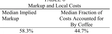
We use equation (14) to derive markups based on the observed wholesale prices and the ran-dom coefficients discrete choice demand system estimated in section 4. Table 6 presents sum-mary statistics on the percentage markup of price over marginal cost implied by this procedure. Throughout this paper, we follow the convention in international economics and define the markup
44
as (p −mc)/mc. The median percentage markup of price over marginal cost is 58.3%. These estimates of the percentage markup are not unusual for consumer packaged goods industries. For example, Nevo (2001) estimates a median markup of about 67% for the ready-to-eat cereal industry. Villas-Boas (2007) estimates wholesale markups in the range of 25−100% for yogurt.45
To obtain estimates of the local costs of production, we simply subtract coffee commodity costs from the total marginal cost (which can be obtained by “inverting” the markup). A small estimated markup therefore implies that local costs must be large to rationalize the observed prices and vice versa. Table 6 presents statistics on the role of coffee beans in marginal costs. On average, coffee beans account for almost half of marginal costs. This fraction is roughly consistent with industry estimates of the magnitude of non-coffee costs reported in Yip and Williams (1985) and the Survey of Manufacturers. These estimates are also similar to Bettendorf and Verboven’s (2000) results for the Dutch coffee market. Since the inputs used to produce an ounce of coffee are relatively stable, the fraction of marginal costs accounted for by coffee beans tends to rise with the commodity cost of coffee. According to the census of manufacturers, green bean coffee accounted for 75% of non-capital costs in 1997 when commodity costs were at a high, but the proportion fell to 43% by 2002 when commodity costs were at a low.
6
A Menu Cost Model of an Oligopoly
The standard static pricing model discussed in the previous section does not account for the in-frequent price adjustments or delayed price responses documented in section 3. In this section, we therefore extend the model to allow for adjustment costs in price-setting. The model builds on previous menu cost models estimated using dynamic methods by Slade (1998, 1999) and Aguirre-gabiria (1999). The model we use is, however, somewhat different from existing menu cost models due to the oligopoly framework. In particular, we allow for small random costs of adjustment, as for example in Dotsey, King, and Wolman (1999). While the distribution of these costs is known, the realization of the menu cost is private information. Incorporating menu costs into the firm’s pricing problem makes the pricing problem fundamentally dynamic. If a cost change is expected to persist for many periods, a forward-looking firm may choose to adjust its prices even if the current benefit from doing so is quite small. Moreover, given the oligopoly setting, the firm recognizes that its competitors may respond in the future to its current pricing decisions.
The model is formally related to the dynamic oligopoly model studied by Pakes and McGuire (1994).46 It is not possible to solve analytically for the Markov perfect equilibrium of the model.
Therefore, we adopt methods from this literature (e.g. Benkard (2004)) to numerically solve for the equilibrium pricing policies of the firms. The equilibrium concept that we adopt is a Markov perfect Nash equilibrium, where the strategy space consists of firms’ prices (Maskin and Tirole,
45
As a check on whether the estimates are reasonable, I also investigated the fraction of implied marginal costs that are negative: we find that negative implied marginal costs occur extremely infrequently—less than 0.2% of the time.
46
1988). This equilibrium concept restricts attention to pay-off relevant state variables, thus focusing attention away from the large number of other subgame perfect equilibria that exist in this type of model.
We use value function iteration to solve for the policies of the individual firms and then use an iterative algorithm to update the firms’ policy functions until a fixed point is achieved. We assume that demand is given by the demand system estimated in section 4. As in the case of the Pakes-McGuire algorithm, there is no guarantee that this algorithm converges.47
6.1 Model
The model consists of a small number of oligopolistic firms. Firmjseeks to maximize the discounted expected sum of future profits,
E0 ∞
X
t=0
βthπjmt(pwmt, Ct)−γjmt1(∆pwjmt6= 0)
i
, (15)
where pw
mt is the vector of wholesale prices (per ounce) in market m at time t, πjmt is the firm’s
per-period profit,Ctis the commodity cost,β is the firm’s discount factor,γjmt is a random menu
cost the firm pays if it changes its prices, and 1(∆pw
jmt6= 0) is an indicator function that equals one
when the firm changes its price. Equation 15 assumes that, though each firm produces multiple products, its pricing decisions across products are coordinated. We discuss this assumption below. Each firm maximizes profits. We assume that β = 0.99. The firm’s profitsπjmt(pwmt, Ct) are given
by expression (11) above, where the relationship between retail and wholesale prices is discussed below. The firm’s profits depend both on its own prices and the prices of its competitors.
The menu costγjmtis independent and identically distributed with an exponential distribution;
i.e., F(γjmt) = 1−exp (−σ1γjmt). The firm’s draw of the menu costγjmtis private information. In
every period, the pricing game has the following structure:
1. Firms observe the commodity costCt and their own draws of the menu costγjmt.
2. Firms choose wholesale prices pw
jmt simultaneously (without observing other firm’s draws of
γjmt).
The Bellman equation for firm j’s dynamic pricing problem is thus,
Vj(pwmt−1, Ct, γjmt) = max pw
jmt
Et
h
πjmt(pwmt, Ct)−γjmt1(∆pjmtw 6= 0) +βVj(pwmt, Ct+1, γjmt+1)
i
, (16)
whereEt is the expectation conditional on all information known by firm j at time tincluding its
own menu costγjmt. The expectation is taken over two sources of uncertainty: uncertainty about
the future commodity costCt+1and uncertainty about competitors’ prices arising because the menu
costs are private information. Notice that a given firm’s profits and value function depend on all firms’ prices through the demand curve. From the perspective of a firm’s competitors, its strategy has two parts. First, the pricing rulepwj (pwmt−1, Ct) for all firmsj = 1, ..., B gives the firm’s priceif
47
it decides to change its price. Second, the probability function prj(pw
mt−1, Ct) gives the probability
that the firm changes its price for a particular value of the publicly observable variables (pwmt−1, Ct).
An equilibrium is defined as a situation where a firm chooses optimal policies (i.e. the Bellman equation (16) is satisfied), and the firm’s expectations are consistent with the equilibrium behavior of the firm’s competitors. As we note above, the firm’s strategy is restricted to be Markov; i.e., to depend only on the payoff-relevant state.
To make the problem computationally tractable, we make the following simplifying assumptions. First, we assume that the prices for different sizes of the same brand move together (i.e., if the per-ounce price of Folgers 16 ounce coffee increases by 10 cents then the same thing happens to the per-ounce price of Folgers 40 ounce coffee). So we have,
pwkmt=pwjmt+αk, (17)
for all k ∈ Υj, where αk is a known parameter. This assumption is motivated by the fact that
empirically, the timing of price changes is often coordinated across products owned by the same brand.48
Second, we assume that retail prices equal wholesale prices plus a known constant margin ξk,
prkmt=ξk+pwkmt. (18)
Marginal cost is modeled as the sum of a product-specific constantµk and the commodity cost,
mckmt=µk+Ct. (19)
This specification is meant to capture the idea that non-coffee costs are several times less variable than coffee commodity costs. By adopting this specification, we also assume that the firm faces constant returns to scale in production.49
Uncertainty about future costs takes the form,
Ct=a0+ρCCt−1+ǫC, (20)
where ǫC is distributed N(0, σ2C) and σC2, a0 and ρC are known coefficients. Since a unit root in
commodity costs cannot be rejected at standard confidence levels, we model commodity costs as a random walk; i.e., a0 = 0 andρC = 1. Firms’ perceptions about the stochastic process of costs
play a key role in determining pass-through, as we discuss in section 7. For computational reasons, we assume that commodity costs follow a random walk so long as costs lie between the boundsCH
and CL, but are bounded within this region.
The firm’s decision about whether to adjust its price depends on the difference between its payoffs when it adjusts and when it does not adjust,
∆W =Wch−Wnch, (21)
48
Conditional on at least one product from a particular brand adjusting in a given month, the probability of adjustment across all products is 93.8% over the 1997-2005 period.
49