Fuzzy P & O Maximum Power Point Tracking Algorithm for a Stand Alone Photovoltaic System Feeding Hybrid Loads

http://dx.doi.org/10.4236/sgre.2014.52003

Fuzzy P & O Maximum Power Point Tracking Algorithm

for a Stand-Alone Photovoltaic System Feeding

Hybrid Loads

Sahar M. Sadek1, Faten H. Fahmy1, Abd El-Shafy A. Nafeh1, Mohamed Abu El-Magd2

1

Electronics Research Institute, National Research Center Building, Cairo, Egypt; 2Faculty of Engineering, Cairo University, Cairo, Egypt.

Email: saharsadek6@yahoo.com

Received October 31st, 2013; revised November 30th, 2013; accepted December 7th, 2013

Copyright © 2014 Sahar M. Sadek et al. This is an open access article distributed under the Creative Commons Attribution License, which permits unrestricted use, distribution, and reproduction in any medium, provided the original work is properly cited. In accor-dance of the Creative Commons Attribution License all Copyrights © 2014 are reserved for SCIRP and the owner of the intellectual property Sahar M. Sadek et al. All Copyright © 2014 are guarded by law and by SCIRP as a guardian.

ABSTRACT

The photovoltaic (PV) generator exhibits a nonlinear current-voltage (I-V) characteristic that its maximum power point (MPP) varies with solar insolation. In this paper, a maximum power point tracking (MPPT) method using fuzzy logic control (FLC) is presented. This method is based on the concept of perturbation and observa-tion (P & O) algorithm to track the MPP of a stand-alone PV system. The controller is used to maximize the power generated by the PV array and the simulation of the system is implemented in MATLAB. Simulation re-sults are compared with those obtained by the conventional P & O controller. Rere-sults show that the FLC gives better and more reliable control for the stand-alone PV system feeding hybrid loads.

KEYWORDS

PV; MPPT; Fuzzy Controller; DC & AC Loads

1. Introduction

Photovoltaic (PV) generation is becoming increasingly important as a renewable source. There is a point on the current-voltage (I-V) or power-voltage (P-V) curves of photovoltaic, called the Maximum power point (MPP), at which PV operates with maximum efficiency and pro-duces its maximum output power [1]. Several power MPPT methods that force the operating point to oscillate have been presented in the past few decades such as 1) perturb and observe (P & O) [2], 2) incremental conduc-tance (Inc Cond) [3], 3) parasitic capaciconduc-tance [1], 4) vol-tage-based peak power tracking [4], and 5) current-based peak power tracking [4]. A significant number of MPPT control schemes have been developed since 1970s, start-ing with simple techniques such as feedback voltage and current MPPT methods. Then, other methods such as the P & O technique or the Inc Cond technique are used to more improve power from PV generator [5]. Recently, intelligence-based control schemes MPPT have been

introduced. The implementation of fuzzy logic is based on the input change of power and input change of power with respect to change of voltage. However, fuzzy can determine the size of perturbed voltage needed to reach MPP [6].

It must be pointed out that all the conventional track-ing methods use fixed, small iteration steps, determined by the accuracy and tracking speed requirements. If the step size is increased to speed up the tracking, the accu-racy of tracking suffers and vice versa. To overcome this limitation, a variable step size method is applied in MPPT of photovoltaic (PV) generation [7].

This paper introduces a maximum power point track-ing (MPPT) method, ustrack-ing fuzzy logic control (FLC) and P & O algorithm, to increase the PV output power in a stand-alone PV system feeding hybrid loads.

2. Proposed PV System

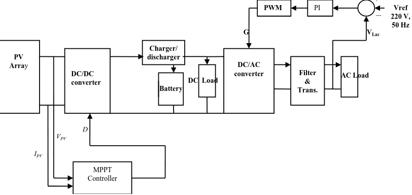
energy storage system and a regulated output voltage source inverter, is proposed in this work, to feed conti-nuous hybrid loads (DC & AC). Figure 1 shows the block diagram of the suggested stand-alone PV system. In the considered photovoltaic system, MPPT tracking control is introduced to maximize the PV output power during the sunshine hours. Noting that, the battery that is charged during the daylight hours is utilized, in this case, to feed the hybrid loads during night hours or during the weak weather conditions.

This system consists of 16 PV modules of 75 WP each.

The array is configured such that the number of modules connected in series is 2 and the number of parallel strings is 8. The battery bank consists of 8 batteries, each has 12 V and 100 Ah, and is configured such that the number of batteries connected in series is 2 and the number of pa-rallel strings is 4. Therefore, the battery bank has a no-minal voltage of 24 V and capacity of 800 Ah.

3. System Modeling

3.1. Photovoltaic Array

In this work, the PV array equivalent circuit model (Figure2) is represented by [8].

( )

(

)

L o

I =I −I e + − (1)

where, I is the PV array current, V is the PV array voltage,

q is the electronic charge, n is the ideality factor, K is the Boltzman’s constant, T is the absolute temperature, Rs is

the array series resistance, IL is the photocurrent and Io is

the array reverse saturation current.

3.2. Battery

The relation between the battery voltage Vb and current Ib

is represented by the Equation (2) [9]

b b b

V = ±E I R (2)

where, E is the battery electromotive force. Also, the “+” sign is used for charging and the “−” one is for discharg-ing.

3.3. Battery Charger/Discharger

The battery charger/discharger is modeled, in this case, with on-off switches that can safely charge or discharge the battery.

3.4. AC Load Interfacing

It consists of a regulated DC/AC inverter, L-C filter and step up transformer to give 220 V at 50 Hz for the AC load.

3.5. Electrical Loads

The stand-alone PV system is designed, in this work, to feed hybrid DC & AC loads with maximum PV power. The DC load is represented by a resistance of 24 V and 60 W. While, the AC load is represented by an R-L load of 220 V (RMS), 50 Hz with 0.8 power factor lagging and 170 W.

4. System Controller

4.1. Conventional P & O Controller

Maximum power tracking P & O algorithm is one of the most successful and commonly used methods because of its simplicity to implement in hardware. This algorithm is applied, in this work, to buck converter. The duty cycle

D of the buck converter changes during the algorithm searches the MPP. At the same time, the corresponding

Figure 1. Block diagram of the stand-alone PV system.

PV Array

DC/DC converter

MPPT Controller

Charger/ discharger

DC Load

IPV VPV

DC/AC

converter Filter

& Trans.

AC Load

－

PI

PWM

G VLac

Vref 220 V, 50 Hz

Battery

D

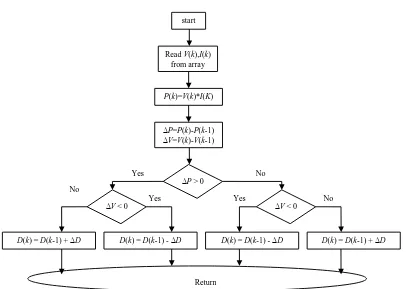
input voltage of converter changes until it reaches its MPP value. The main drawback of this method is the waste of energy in steady state conditions especially at low irradiations. Figure 3 shows the flow chart of the conventional P & O algorithm [10]. Thus, this algorithm shows that if the current PV generated power P k

( )

(

)

0

V

∆ > , the voltage is increased; this is done through

( )

(

)

D k =D k− +C (C, incrimination step) when

0

V

∆ > , the voltage is decreased through

( )

(

)

D k =D k− −C.

4.2. P & O Fuzzy Logic Controller

Fuzzy logic controllers have the advantages of working with imprecise inputs, not needing an accurate mathe-matical model, and handling nonlinearity. Fuzzy logic control generally consists of three stages: fuzzification, rule evaluation, and defuzzification [11]. During fuzzifi-cation, numerical input variables are converted into lin-guistic variables based on a membership function similar to Figure4. In most fuzzy controllers, the two inputs are error (E) and change of error (CE); where, E is ∆ ∆P V

and CE=E k

( )

(

)

The rule evaluation uses the fuzzified output from the fuzzification stage and the rules from the rule base to

produce the fuzzy output variable. The defuzzification stage converts the fuzzy output variable that is produced from the rule evaluation into a single real number. In this case, seven fuzzy sets are used for inputs and output as shown in Table 1 where, NB stands for negative big,

Table 1. Rules base of fuzzy logic controller.

∆V

∆P NB NM NS ZE PS PM PB

NB NB NB NB NB NM NS ZE

NM NB NB NB NM NS ZE PS

NS NB NB NM NS ZE PS PM

ZE NB NM NS ZE PS PM PB

PS NM NS ZE PS PM PB PB

PM NS ZE PS PM PB PB PB

PB ZE PS PM PB PB PB PB

Figure 2. PV equivalent circuit model.

Figure 3. Flow chart of P & O algorithm.

IL

V IO

I RS G

T

start

Read V(k),I(k)

from array

P(k)=V(k)*I(K)

∆P=P(k)-P(k-1)

∆V=V(k)-V(k-1)

∆P> 0

∆V< 0 ∆V< 0

D(k) = D(k-1) + ∆D

D(k) = D(k-1) + ∆D D(k) = D(k-1) -∆D D(k) = D(k-1) -∆D

Return Yes

No

Yes Yes

No

NM for negative medium, NS for negative small, ZE for zero, PS for positive small, PM for positive medium and PB for positive big. The rules base of this fuzzy logic controller is presented in this table. In this work, the in-puts of the designed fuzzy logic controller can be simpli-fied by using ∆V and ∆P according to the same P & O concept, while the output is the duty cycle ∆D. The following equations show the inputs to FLC.

( )

(

)

P p k P k

∆ = − − (3)

( )

(

)

V V k V k

∆ = − − (4)

As an example, for a certain control rule from Table1, if ∆P is PB and ∆V is ZE THEN ∆D is PB. This implies that if the operating point is distant from MPP towards left hand side and the change in voltage is about zero, then the controller should increase the duty ratio largely for reaching the MPP.

5. Simulation Results

Each subsystem of the stand-alone PV system is modeled and simulated in MATLAB environment. Then, a com-bination between subsystems gives a complete simula-tion model. In this paper, the results show the compari-son between the conventional P & O MPPT controller and the modified one that uses the FLC and validate their corresponding effect on PV array output power. The bat-tery bank power performance, DC load and AC load performances are shown by the results of simulation at insolation data of sunny and cloudy days for Kharga Oa-

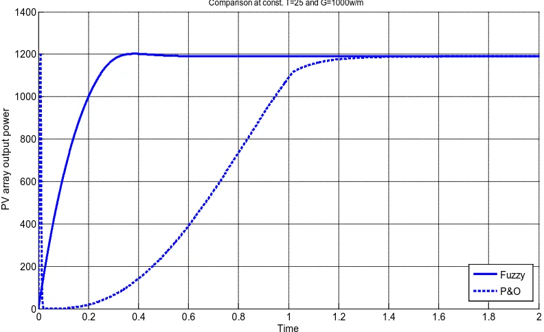
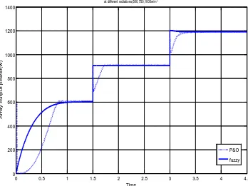
sis that is a location in west Egypt. Figure 5 shows the dynamic response of the PV output power at constant insolation level of 1000 W/m2 and at constant tempera-ture of 25˚C. Figures6 and 7 show the dynamic perfor-mance of the PV output power at constant temperature of 25˚C and at sudden decrease and increase in insolation level, respectively. Figure8 shows the response of the PV array output power at steady state conditions while the insolation is relatively low (600 W/m2). Zooming on the curve shows the oscillation of power in case of using the conventional P & O method. These figures indicate that using the FLC based on the P & O method can give the system a very fast response for MPPT (with nearly no oscillations on the MPP at steady state).

The overall stand-alone PV system simulation model was run two times at a sunny day and a cloudy day ac-cording to the location represented before. Results are exhibited in three groups to show the performances of

Figure 4. Membership function for inputs (∆V & ∆P) and

output (∆D).

Figure 5. Array output power with P & O and FLC.

0 0.2 0.4 0.6 0.8 1 1.2 1.4 1.6 1.8 2

0 200 400 600 800 1000 1200 1400

Time

P

V

ar

ray

out

put

pow

er

Comparison at const. T=25 and G=1000w/m2

Fuzzy

P&O

Figure 6. Array output power with P & O and FLC.

Figure 7. Array output power with P & O and FLC.

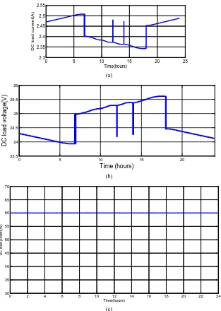
DC load, AC load and battery after using the FLC MPPT controller instead of the conventional P & O MPPT con-troller. The output currents of DC & AC loads are pre-sented by (ILdc, ILac), output load voltages (VLdc, VLac), DC

load power (PLdc) and the root mean square value of the

AC load power (PLac-RMS). Figures9 and 10 show the

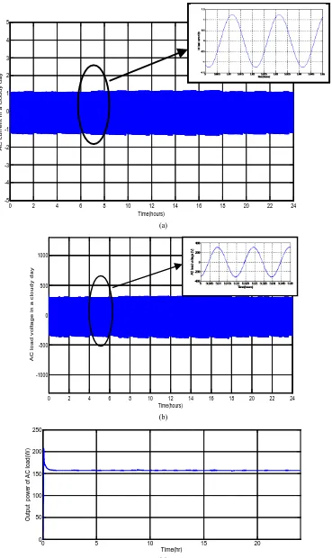
performances of DC load for cloudy and sunny days re-spectively. Figures11 and 12 show the performances of

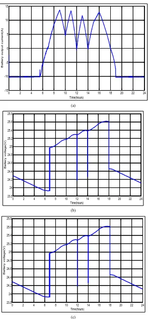
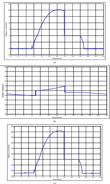
AC load in cloudy and sunny days with zooming on the AC load current and voltage to show the 220 V and 50 Hz output values. The AC load output power is presented as a RMS value. Figures 13 and 14 show the perfor-mance of the battery in cloudy & sunny days. It can be shown that the battery takes charging time with MPPT controller of eight hours and capable of supplying the full load up to eleven hours, where Vb is the battery voltage,

0 0.5 1 1.5 2 2.5 3 3.5 4 4.5

0 200 400 600 800 1000 1200 1400

Time

A

rr

ay

out

put

pow

er

(w

)

Comparison of P&O and FLC at decreasing Rad.

fuzzy P&o

0 0.5 1 1.5 2 2.5 3 3.5 4 4.5

0 200 400 600 800 1000 1200 1400

Time

A

rr

ay

out

put

pow

er

(w

)

at different radiations(500,750,1000w/m2

P&O

fuzzy

Figure 8. Zoom on array output power with P & O and FLC.

(a)

(b)

(c)

Figure 9. Performance of DC load during cloudy day. (a) Load current, (b) Load voltage, (c) Load power.

0 0.5 1 1.5 2 2.5 3

0 100 200 300 400 500 600 700 800

Time

O

ut

put

P

V

ar

ray

pow

er

(W

)

1.5 1.55 1.6 1.65 1.7 1.75 1.8 1.85 1.9 1.95 2 728

728.5 729 729.5 730 730.5 731

Time

O

ut

put

P

V

ar

ray

pow

er

(W

)

0 5 10 15 20 25

2.3 2.35 2.4 2.45 2.5 2.55

Time(hours)

D

C

l

oad c

ur

rent

(A

)

0 5 10 15 20

23.5 24 24.5 25 25.5 26

Time (hours)

D

C

l

oad v

ol

tage(

V

)

0 2 4 6 8 10 12 14 16 18 20 22 24

30 35 40 45 50 55 60 65 70

Time(hours)

D

C

load pow

er

(W

(a)

(b)

(c)

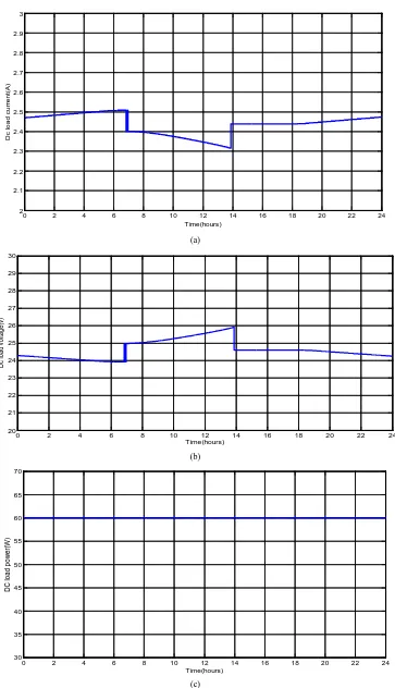
Figure 10. Performance of DC load during sunny day. (a) Load current, (b) Load voltage, (c) Load power.

0 2 4 6 8 10 12 14 16 18 20 22 24

2 2.1 2.2 2.3 2.4 2.5 2.6 2.7 2.8 2.9 3

Time(hours)

D

c

l

oad c

ur

rent

(A

)

0 2 4 6 8 10 12 14 16 18 20 22 24

20 21 22 23 24 25 26 27 28 29 30

Time(hours)

D

c l

oad v

ol

tage(

v)

0 2 4 6 8 10 12 14 16 18 20 22 24

30 35 40 45 50 55 60 65 70

Time(hours)

D

C

load pow

er

(W

(a)

(b)

(c)

Figure 11. Performance of AC load during a cloudy day. (a) Load current; (b) Load voltage; (c) Load power.

0 2 4 6 8 10 12 14 16 18 20 22 24

-5 -4 -3 -2 -1 0 1 2 3 4 5

Time(hours)

A

C

c

u

rr

e

n

t i

n

a c

lou

d

y

d

a

y

0 2 4 6 8 10 12 14 16 18 20 22 24

-1000 -500 0 500 1000

Time(hours)

A

C

l

oad v

ol

tage i

n a c

loudy

day

0 5 10 15 20

0 50 100 150 200 250

Time(hr)

O

ut

put

pow

er

of

A

C

l

oad(

W

(a)

(b)

(c)

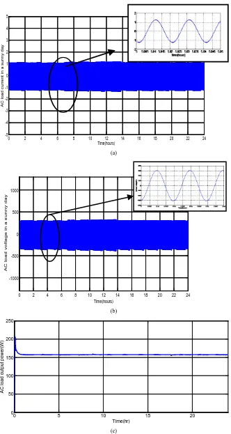
Figure 12. Performance of AC load during a sunny day. (a) Load current; (b) Load voltage; (c) Load power.

0 2 4 6 8 10 12 14 16 18 20 22 24

-5 -4 -3 -2 -1 0 1 2 3 4 5

Time(hours)

A

C

l

o

ad

c

ur

r

e

nt

i

n

a s

u

n

ny

d

ay

0 2 4 6 8 10 12 14 16 18 20 22 24

-1000 -500 0 500 1000

Time(hours)

A

C

l

oad v

ol

tage i

n a s

unny

day

0 5 10 15 20

0 50 100 150 200 250

Time(hr)

A

C

l

oad out

put

pow

er

(W

(a)

(b)

(c)

Figure 13. Performance of battery during a cloudy day. (a) Battery current; (b) Battery voltage; (c) Battery power.

0 2 4 6 8 10 12 14 16 18 20 22 24

-15 -10 -5 0 5 10 15

Time(hours)

B

at

ter

y

out

put

c

ur

rent

(A

)

0 2 4 6 8 10 12 14 16 18 20 22 24

23.8 24 24.2 24.4 24.6 24.8 25 25.2 25.4 25.6 25.8

Time(hours)

B

at

ter

y

v

ol

tage(

V

)

0 2 4 6 8 10 12 14 16 18 20 22 24

23.8 24 24.2 24.4 24.6 24.8 25 25.2 25.4 25.6 25.8

Time(hours)

B

at

ter

y

v

ol

tage(

V

(a)

(b)

(c)

Figure 14. Performance of battery during a sunny day. (a) Battery current; (b) Battery voltage; (c) Battery power.

0 2 4 6 8 10 12 14 16 18 20 22 24

-15 -10 -5 0 5 10 15 20 25

Time(hours)

B

at

ter

y

c

ur

rent

(A

)

0 2 4 6 8 10 12 14 16 18 20 22 24

20 21 22 23 24 25 26 27 28 29 30

Time(hours)

B

at

ter

y v

ol

tage(

V

)

0 2 4 6 8 10 12 14 16 18 20 22 24

-300 -200 -100 0 100 200 300 400 500 600

Time(hours)

B

at

ter

y

pow

er

(W

Ib is its current and Pb is the power output of the battery.

6. Conclusion

A simulation model is designed for a stand-alone PV system feeding continuous hybrid (DC & AC) loads. The system is controlled by conventional P & O controller and then by FLC; for extracting the maximum power from the PV array. The system is simulated in MATLAB software. In the proposed algorithm the fixed perturba-tion step size deficiency is overcome through using FLC which is designed to determine the suitable (variable) perturbation step size. Results of comparison of these two controllers in the PV system show adequate and ro-bust performance for the proposed FLC in terms of rise time, settling time and steady state error. Thus, The FLC enables the PV system to reach the MPP faster and with fewer fluctuations at steady state conditions. This means that the FLC is able to improve the amount of energy extracted from PV array. At the same time, the results show that the PV system with FLC can feed the battery and loads with better performance at all climatic varia-tions.

REFERENCES

[1] H. E. A. Ibrahim and M. Ibrahim, “Comparison between Fuzzy and P&O Control for MPPT for Photovoltaic Sys-tem Using Boost Converter,” Journal of Energy Tech-nologies and Policy, Vol. 2, No. 6, 2012, p. 1.

[2] X. Liu and L. A. C. Lopes, “An Improved Perturbation and Observation Maximum Power Point Tracking Algo-rithm for PV Arrays,” 35th Annual IEEE Power Elec-tronics Specialist’s Conference, Aachen, 20-25 June 2004, pp. 2005-2010.

[3] D. P. Hohm and M. E. Ropp, “Comparative Study of Maximum Power Point Tracking Algorithms Using An Experimental, Programmable, Maximum Power Point Tracking Test Bed,” 28th IEE Photovoltaic Specialist

Conference, Anchorage, 2000, pp. 1699-1702. http://dx.doi.org/10.1109/PVSC.2000.916230

[4] A. S. Mohammad, et al., “Theoretical and Experimental Analyses of Photovoltaic Systems with Voltage- and Current-Based Maximum Power-Point Tracking,” IEEE Transactions on Energy Conversion, Vol. 17, No. 4, 2002, pp. 514-521. http://dx.doi.org/10.1109/TEC.2002.805205

[5] V. Salas, et al., “Review of the Maximum Power Point Tracking Algorithms for Stand-Alone Photovoltaic Sys- tems,” Solar Energy Materials & Solar Cells, Vol. 90, No. 11, 2006, pp. 1555-1578.

http://dx.doi.org/10.1016/j.solmat.2005.10.023

[6] C. S. Chin, P. Neelakantan, H. P. Yoong and K. T. K. Teo, “Control and Optimization of Fuzzy Based Maximum Power Point Racking in Solar Photovoltaic System,” Glo- bal Conference on Power Control and Optimization, Ku- ching, 2-4 December 2010.

[7] J. Y. Li and H. H. Wang, “A Novel Stand-Alone PV Generation System Based on Variable Step Size INC MPPT and SVPWM Control,” IEEE 6th International of Power Electronics and Motion Control Conference, Wu-han, 17-20 May 2009, pp. 2155-2160.

[8] G. Walke, “Evaluation MPPT Converter Topologies Us- ing A MATLAB Photovoltaic Model,” Journal of Elec-trical & Electronic Engineering Australia, Vol. 21, No. 1, 2001, pp. 49-56.

[9] L. Castaner and S. Silvestre, “Modeling PV Systems Us-ing Pspice,” John Wiley & Sons Ltd., 2002.

http://dx.doi.org/10.1002/0470855541

[10] H. Knopf, “Analysis, Simulation and Evaluation of Maxi- mum Power Point Tracking (MPPT) Methods for a Solar Powered Vehicle,” Master Thesis, Portland State Univer-sity, 1999.

[11] R. Rahmani, M. Seyedmahmoudian, S. Mekhilef and R. Yusof, “Implementation of Fuzzy Logic Maximum Power Point Tracking Controller for Photovoltaic System,” Ame- rican Journal of Applied Sciences, Vol. 10, No. 3, 2013, pp. 209-218.