MCMC for integer valued ARMA processes

MCMC for integer valued ARMA processes

Peter Neal

_{and T. Subba Rao}

University of Manchester

June 7, 2006

Address:

Mathematics Department,

University of Manchester,

Sackville Street,

PO Box 88,

Manchester,

M60 1QD,

UK

E-mail: [email protected]

Abstract

The Classical statistical inference for integer valued time-series has primarily been restricted to

the integer valued autoregressive (INAR) process. Markov chain Monte Carlo (MCMC) methods have

been shown to be a useful tool in many branches of statistics and is particularly well suited to integer

valued time-series where statistical inference is greatly assisted by data augmentation. Thus in the

current work, we outline an efficient MCMC algorithm for a wide class of integer valued

autoregres-sive moving-average (INARMA) processes. Furthermore, we consider noise corrupted integer valued

processes and also models with change points. Finally, in order to assess the MCMC algorithms

inferential and predictive capabilities we use a range of simulated and real data sets.

Keywords: Integer valued time-series, MCMC, count data.

1

Introduction

Integer valued time-series occur in many different situations, and often in the form of count data.

Con-ventional time-series models such as the standard univariate autoregressive moving-average (ARMA)

process with Gaussian errors, assume that the data take values in R. Therefore these standard models

are wholely inappropriate for integer valued time-series, especially for low frequency count data where

continuous approximations of the discrete process are particularly unsuitable (see, for example,

Free-land and McCabe (2004) and McCabe and Martin (2005).) Hence there has been considerable interest

in developing and understanding time-series models which are suitable for integer valued processes, see

McKenzie (2003), for an excellent review of the subject. This has led to the construction of integer

valued ARMA (INARMA) processes, and alternatives such as discrete ARMA (DARMA) processes (see,

McKenzie (2003) for a description of the model). Throughout this paper we shall focus on INARMA

processes, with a full description being given in Section 2.

Whilst INARMA processes have received a certain amount of attention over the last twenty-five years,

they are considerably less well understood and analysed than the standard ARMA processes. In

par-ticular, inference for the model parameters governing the INARMA process has received very limited

attention. Attention has almost exclusively been restricted to INAR(1) processes, both for classical

frequentist inference (see, for example, Franke and Seligmann (1993)) and Bayesian inference (see, for

example, Freeland and McCabe (2004) and McCabe and Martin (2005)). Although recently Jung and

Tremayne (2006) have considered an INAR(2) process. This is due to the complicated form of the

such problems is given in Daviset al. (2000), where a Poisson regression model is used with a standard

ARMA(p,q) time-series forming part of the underlying latent process. Our approach differs radically

from Daviset al. (2000), in that, we define the process directly in terms of a time-series model, namely

the INARMA(p, q) model. To this end MCMC (Markov chain Monte Carlo) greatly assists since MCMC

easily incorporates data augmentation which facilitates inference for such models (see, Gilkset al.(1996),

for a good introduction to the MCMC methodology). Thus we are able to tackle, relatively easily a wide

range of time-series models which is a considerable improvement on classical approaches taken in Franke

and Seligmann (1993), Freeland and McCabe (2004), McCabe and Martin (2005) and Jung and Tremayne

(2006). Note that MCMC has previously been used to tackle a number of time-series problems, see for

example, Troughton and Godsill (1997) and Daniels and Cressie (2001).

In analysis of time series data, we are interested, typically, either in the underlying model parameters or

the predictive capabilities of the model, or both. Therefore the aim of the current work is to establish

a mechanism for conducting inference for both the model parameters and the predictive conditional

distribution for a wide range of INARMA processes and their extensions, via MCMC. MCMC is primarily,

but not exclusively, used for inference in a Bayesian framework, and in this paper we shall take a Bayesian

approach.

In Section 2, the INARMA process is introduced and some extensions of the model are discussed. In

Section 3, the likelihood function for the INARMA process is derived, and this is analysed using an

MCMC algorithm which we give full details of. This leads to analysis of the data in Section 4. Firstly

simulated data and then real life data are used to assess both the capabilities of the MCMC algorithm

and of the model. The first real life data set is Westgren’s gold particle data set (Westgren (1916)) which

has recently been analysed in Jung and Tremayne (2006). The second real life data set concerns the

daily scores achieved by a schizophrenic patient on a test of perceptual speed, McCleary and Hay (1980).

The patient begins receiving a drug during the course of the study and therefore a change point model

is used to assess the affect of the drug on the patient’s test scores. Finally, in Section 5 we make some

2

Models

2.1

Integer-valued ARMA processes

An integer valued time-series {Xt;−∞< t <∞} is called an INARMA(p, q) process, if it is an integer

valued autoregressive moving-average process with orders p and q, respectively. The INARMA(p, q)

process is given by the following difference equation:

Xt=

p

X

i=1

αi◦Xt−i+ q

X

j=1

βj◦Zt−j+Zt, t∈Z, (2.1)

for some generalised, Steutel and van Harn, operatorsαi(1≤i≤p) andβj (1≤j≤q) (see, Steutel and

van Harn (1979) and Latour (1997)) andZt(−∞< t <∞) are independent and identically distributed

according to an arbitrary, but specified, non-negative integer valued random variable Z with E[Z2] <

∞. Furthermore the operators are all assumed to be independent. Whilst INAR(p) (integer-valued

autoregressive) processes are defined and analysed in Latour (1997) for generalised Steutel and van Harn

operators, we shall, for clarity of presentation of the results, restrict attention to binomial operators. The

binomial operator,γ◦, for a non-negative integer-valued random variable,W say, is defined as

γ◦W =

 



Bin(W, γ) W >0,

0 W = 0.

That is, the operator γ denotes the ‘success’ probability for the binomial distribution. Clearly for a

binomial operator γ, 0 ≤ γ ≤ 1. The binomial operator is chosen because it is the natural choice of

generalised Steutel and van Harn operator in many different situations. (Furthermore, the binomial

operator is the operator considered in Steutel and van Harn (1979).) However, most of the results and

procedures presented here readily extend to more general, generalised Steutel and van Harn operators

with the minimum of fuss.

To ensure that the above INARMA(p, q) process is (second-order) stationary, we require that α =

(α1, α2, . . . , αp) are such that the roots of thep-order polynomial

xp−α1xp

−1₋

. . .−αp−₁x−α_p= 0

are inside the unit circle (see, Latour (1997)). We shall, however, use the stronger, but easier to check

cri-terion thatPp

i=1αi<1, to ensure that the process is stationary. Note the parallels with the requirements

for stationarity of a real-valued ARMA process. We shall also add a constraint forβ= (β1, β2, . . . , βq),

in that, we shall assumePq

time series to be invertible. It is an open question whether this condition is sufficient for the INARMA

process to be invertible.

One natural extension of the INARMA(p, q) process is the inclusion of a noise term, Dt say. Let

{Wt;−∞< t <∞} denote an INARMA(p, q) process with noise, then

Wt=Xt+Dt, t∈Z, (2.2)

where {Xt} is INARMA(p, q) process of the form (2.1) and Dt (−∞ < t < ∞) are independent and

identically distributed non-negative integer-valued random variables. Furthermore, we assume that the

two processes {Xt;−∞< t <∞} and{Dt;−∞< t <∞} are independent. Throughout this paper we

assumeZtandDtare Poisson distributed for succinctness, however, it is straightforward in principle to

consider alternative integer valued distributions.

2.2

Data

We naturally restrict attention to non-negative integer valued time series data, typically this will take the

form of count data. We shall assume that we observe part of the time series and that the data is complete

for the section of the time series observed. However, the methodology outlined in Section 3 can easily be

extended to incorporate missing data, by considering the missing data as extra parameters which are to

be imputed within the model. For the INARMA(p, q) process we assume that the data (observed

time-series) arex = (x1−_r, x2−_r, . . . , x_n) wherer = max{p, q} for somen ≥1. For the INARMA(p, q) with

additive noise, the data comprisesw= (w1−_r, w2−_r, . . . , w_n) for some n≥1. Without loss of generality,

we shall assume thatn > r.

3

Likelihood and MCMC algorithms

3.1

Likelihood of INARMA

(

p, q

)

process

For conciseness, throughout this section we shall assume thatZ ∼P o(λ). Also we assume that the orders

pandqof INARMA(p, q) are known withp, q >0. (The procedure simplifies considerably if eitherp= 0

orq= 0.) Thus, we have an observed time seriesx= (x1−r, x2−r, . . . , xn) wherer= max{p, q}. We are

then interested in inference for the parametersα,β andλwhich are assumed to be unknown. Inference

for them-step ahead predictive distribution,Xpred

In order to facilitate inference for the INARMA(p, q), it is necessary to augment the data as follows. For

t∈Z, we representαi◦Xt−_i (1≤i≤p) andβ_j◦Z_t−_j (1≤j ≤q) by Y_t,i andV_t,j, respectively. Thus

fort∈Z, we have that

Zt=Xt−

p

X

i=1

Yt,i− q

X

j=1

Vt,j.

For t ∈ Z, let Y_t = (Yt,1, Yt,2, . . . , Yt,p) with Y = (Y1,Y2, . . . ,Yn), let Vt = (Vt,1, Vt,2, . . . , Vt,q)

with V = (V1,V2, . . . ,Vn) and let Zt = (Z1, Z2, . . . , Zt). For t ≥ 1, let yt = (yt,1, yt,2, . . . , yt,p)

and vt = (vt,1, vt,2, . . . , vt,q) with y = (y1,y2, . . . ,yn) and v = (v1,v2, . . . ,vn). For q ≥ 1, let

zIN= (z1−_q, z₂−_q, . . . , z₀), thusz_INrepresents the initial values ofZ, and fort≥1, letz_t= (z₁, z₂, . . . , z_t)

withz0corresponding to the empty set.

Note that given (z_IN,z_t−1,xt−1,α,β, λ) each of the components (Vt,Yt, Zt) are independent, where

xs= (x1−r, x2−r, . . . , xs) (s≥0). Thus fort≥1,

ft(vt,yt, zt|zIN,zt−₁,x_t−₁,α,β, λ)

= ft(zt|zIN,zt−1,xt−1,α,β, λ)×    q Y j=1

ft(vt,j|zIN,zt−1,xt−1,α,β, λ)    × ( p Y i=1

ft(yt,i|zIN,zt−₁,x_t−₁,α,β, λ)

)

= λ

zt zt!

e−_λ

×

p

Y

i=1 ½µ

xt−_i

yt,i

¶

αyt,i

i (1−αi)xt−i

−_yt,i

¾ × q Y j=1 ½µ

zt−_j

vt,j

¶

βvt,j

j (1−βj)zt−j

−_vt,j

¾

. (3.1)

Since by Bayes’ Theorem

ft(vt,yt, zt|xt,zIN,zt−₁,x_t−₁,α,β, λ)

= ft(xt|vt,yt, zt,zIN,zt−1,xt−1,α,β, λ)

ft(xt|zIN,zt−1,xt−1,α,β, λ)

ft(vt,yt, zt|zIN,zt−1,xt−1,α,β, λ), (3.2)

it follows from (3.1) and (3.2) that fort≥1,

ft(vt,yt, zt|x,zIN,zt−₁,α,β, λ)

∝ λ

zt zt!

e−_λ

×

p

Y

i=1 ½µ

xt−_i

yt,i

¶

αyt,i

i (1−αi)xt−i

−_yt,i

¾ × q Y j=1 ½µ

zt−_j

vt,j

¶

βvt,j

j (1−βj)zt−j

−_vt,j

¾

,

subject to the constraints zt+Pp_i=1yt,i+Pq_j=1vt,j = xt, vt,j ≤ zt−_j (1 ≤ j ≤ q) and y_t,i ≤ x_t−_i

(1≤i≤p). Otherwiseft(vt,yt, zt|x,zIN,zt−₁,α,β, λ) = 0. Thus,

f(v,y,zn|x,zIN,α,β, λ) = n

Y

t=1

However, the parametersα,β,λandzIN are unknown. Thus in a Bayesian framework it is necessary to

assign priors to each of these parameters. The parametersα,βandλare assigned the following natural,

independent priors;

π(α)∝1; 0≤αi<1 (1≤i≤p),

p

X

i=1

αi<1;

π(β)∝1; 0≤βj<1 (1≤j≤q),

q

X

j=1

βj <1;

π(λ)∼Gam(Aλ, Bλ); for some Aλ, Bλ>0.

Therefore we have uninformative, uniform priors over the permissable parameter values for the parameters

α andβ and a conjugate Gamma prior forλ. For 1−r≤t≤0, we takeπ(zt|λ,x)∼P o(λ) subject to

the constraint thatzt ≤xt sincea prioriZt is Poisson distributed with meanλ, but also by definition

zt≤xt.

Thus, the full joint likelihood of (V,Y,Zn,ZIN,α,β, λ) given the datax, is given by,

f(v,y,zn,zIN,α,β, λ|x) =f(v,y,zn|zIN,α,β, λ,x)π(α)π(β)π(zIN|λ,x)π(λ).

Therefore it follows that

f(v,y,z,zIN,α,β, λ|x) ∝ n

Y

t=1 (

λzt zt!

e−_λ

p

Y

i=1

½µ_x

t−_i

yt,i

¶

αyt,i

i (1−αi)xt−i

−_yt,i

¾ × q Y j=1 ½µ

zt−_j

vt,j

¶

βvt,j

j (1−βj)zt−j

−_vt,j

¾  



λAλ_e−Bλλ

r

Y

i=1 ½

λz1−i z1−_i!

e−_λ

¾ (3.3)

subject to the aforementioned constraints. The following posterior distributions are then readily obtained

from (3.3):

π(αi|v,y,zn,zIN,αi−,β, λ,x)∼Beta

à 1 +

n

X

t=1

yt,i,1 + n

X

t=1

(xt−_i−y_t,i)

!

(1≤i≤p), (3.4)

whereαi−= (α1, . . . , αi−1, αi+1, . . . αp) and subject to the constraint thatPαk<1;

π(βj|v,y,zn,zIN,α,βj−, λ,x)∼Beta

à 1 +

n

X

t=1

vt,j,1 + n

X

t=1

(zt−j−vt,j)

!

(1≤j ≤q), (3.5)

whereβ_j−= (β1, . . . , βj−₁, β_j+1, . . . β_q) and subject to the constraint that

P

βl<1; and

π(λ|v,y,zn,zIN,α,β,x)∼Gam

Ã

Aλ+

n

X

t=1−q

zt, Bλ+n+q

!

3.2

MCMC algorithm

We are now in a position to outline the MCMC algorithm.

1. Update α: One component at a time, either in a fixed or random order. We sampleαi using the

following Gibbs/rejection sampling procedure:

(i) Draw a proposed value forαi from the Beta distribution given in (3.4);

(ii) If αi is drawn such that Pαk <1, accept the proposed value of αi, and update the value of

αi. Otherwise repeat step (i).

2. Update β: One component at a time, either in a fixed or random order. We sampleβj using the

following Gibbs/rejection sampling procedure:

(i) Draw a proposed value forβj from the Beta distribution given in (3.5);

(ii) Ifβj is drawn such thatPβl<1, accept the proposed value ofβj, and update the value ofβj.

Otherwise repeat step (i).

3. Update λ: Sampleλfrom its conditional distribution given by (3.6).

4. Update (v,y,zn): One set of components (vt,yt, zt) at a time, either in a fixed or random order.

We use the following independence proposal Metropolis-Hastings procedure:

(i) For 1≤i≤p, drawy′

t,i from Bin(xt−_i, α_i);

(ii) For 1≤j ≤q, drawv′

t,j from Bin(zt−_j, β_j);

(iii) Ifxt<Pqj=1v

′

t,j+

Pp

i=1y

′

t,i, then repeat steps (i) and (ii);

(iv) Setz′

t=xt−

³

Pq

j=1v

′

t,j+

Pp

i=1y

′

t,i

´ ;

Thus the proposal distribution for (v′

t,y

′

t, z

′

t) is independent of (vt,yt, zt) and depends only upon

(x,zIN,zt−₁,α,β). Therefore let q_t(v

′

t,y

′

t, z

′

t|x,zIN,zt−₁,α,β) denote the conditional proposal

probability for (v′

t,y

′

t, z

′

t) given (x,zIN,zt−₁,α,β).

(v) Calculate the acceptance probability,A, for the move:

A= 1∧f(v

′

,y′

,z′

n|x,zIN,α,β, λ)

f(v,y,zn|x,zIN,α,β, λ)

×qt(vt,yt, zt|x,zIN,zt−1,α,β)

qt(v′t,y

′

t, z

′

t|x,zIN,zt−₁,α,β)

(3.7)

Note that for s6=t, (v′

s,y

′

s, z

′

s) = (vs,ys, zs). Thus the proposal distribution has been chosen in

have that

A= 1∧zt!

z′

t!

λzt′−zt_B

t,

where Bn= 1 and for 1≤t≤n−1,

Bt=

 



Qq∧_(n−_t)

j=1

n_z′

t!(zt−vt+j,j)!

zt!(z′t−vt′+j,j)!(1−βj)

z′

t−zt

o

if z′

t≥vt+j,j (1≤j≤q∧(n−t)),

0 otherwise.

Therefore if the move is accepted, set (v_t,y_t, zt) equal to (v

′

t,y

′

t, z

′

t), otherwise leave (vt,yt, zt)

unchanged.

5. UpdatezIN: One component at a time, either in a fixed or random order. The procedure to update

zt (1−q≤t≤0) is as follows:

(i) Drawz′

tfrom P o(λ);

(ii) Ifz′

t> xt, repeat step (i);

Thus the proposal probability is

q(z′

t|λ,x) =

π(z′

t|λ)

Fλ(xt)

where Fλ(·) denotes the cumulative distribution function of a Poisson random variable with mean

λ.

(iii) Calculate the acceptance probability,A, for the move:

A = 1∧f(v,y,zn|x,z

′

IN,α,β, λ)π(z

′

t|λ)

f(v,y,zn|x,zIN,α,β, λ)π(zt|λ)

×q(zt|λ,x)

q(z′

t|λ,x)

=  



1∧Qq

j=1−_t

n

z′

t!(zt−_vt+j,j)!

zt!(zt′−vt′+j,j)!(1−βj)

z′

t−zt

o

if z′

t≥vt+j,j (1−t≤j ≤q),

0 otherwise.

Thus we have outlined an MCMC algorithm to obtain samples from the posterior distributions of both

the model parameters (α,β, λ) and the augmented data (v,y,zn,zIN). Typically, we restrict attention

to the posterior distribution of the model parametersπ(α,β, λ|x) which is easily obtained from the above

algorithm.

In the analysis of time series data, we are often interested in the predictive capabilities of the model. In a

Bayesian context, we are interested in them-step ahead predictive distribution,Xpred_m , that is,π(xpred_m |x)

wherexpred_m = (xn+1, xn+2, . . . , xn+m). Clearly,

π(xpred_m |x) =

Z 1 0 Z 1 0 Z ∞ 0 X k X l

π(xpred_m |α,β, λ,zIN=k,zn =l,x)

Thus to obtain samples fromXpred_m , the MCMC algorithm can easily be extended as follows.

6. UpdateXpred_m : One component at a time, sequentially fromxn+1through toxn+m. For 1≤k≤m,

draw zn+k ∼P o(λ),yn+k,i∼Bin(xn+k−_i, α_i) (1≤i≤p) andv_n+k,j ∼Bin(z_n+k−_j, β_j) (1≤j ≤

q). Then set,

xn+k =zn+k+ p

X

i=1

yn+k,i+ q

X

j=1

vn+k,j.

Thus we have sampled (zn+k, xn+k) from its conditional distribution,

π(zn+k, xn+k|α,β, λ,zn,zIN,x,xpred_k−1).

Therefore from step 6 of the algorithm it is trivial to obtain a sample form the posterior, predictive

distribution,Xpred_m ,π(xpred_m |x).

3.3

INAR

(

p

)

+ Noise

We restrict attention to INAR(p) processes with Poisson noise,Dt∼P o(µ), for ease of exposition. The

major difference from the standard INAR(p) process is that the output x = (x1−p, x2−p, . . . , xn) from

the INAR process is unobserved, thus we augment the data by includingx. Note that givenx, we obtain

d= (d1−_p, d₂−_p, . . . , d_n) sincew_t=x_t+d_t.

Suppose thatα,λ,µandxare known. Then, for t≥1,

ft(dt,yt, zt|w,x,α, λ, µ)∝

λzt zt!

e−_λµ

dt dt!

e−_µ

p

Y

i=1

µ_x

t−_i

yt,i

¶

αyt,i

i (1−αi)xt−i

−_yt,i

.

subject to the constraints dt = wt−xt, Ppi=1yt,i+zt = xt and yt,i ≤ xt−_i (1 ≤ i ≤ p). Otherwise

f(dt,yt, zt|w,x,α, λ, µ) = 0. Thus

f(d,y,zn|w,x,α, λ, µ) = n

Y

t=1

ft(dt,yt, zt|w,x,α, λ, µ),

Forα and λ we use the same prior as in Section 3.1. However, we now also require a prior for µ. For

conjugacy, we set π(µ)∼Gam(Aµ, Bµ) for someAµ, Bµ>0. Therefore the posterior distribution forµ

is:

π(µ|w,d,x,y,zn,α, λ)∼Gam

Ã

Aµ+

n

X

t=1−_p

dt, Bµ+n+p

!

. (3.8)

The MCMC algorithm described in Section 3.2 can easily be adapted to include the noise term. The

q= 0). Thus all that is required is to outline the procedure for updating the parameters (x,d, µ). For

simplicity in exposition, letxn = (x1, x2, . . . , xn) (dn = (d1, d2, . . . , dn)) andxIN = (x1−_p, x₂−_p, . . . , x₀)

(dIN = (d1−_p, d₂−_p, . . . , d₀)), so that x = (x_IN,x_n) (d = (d_IN,d_n)). The following steps should be

appended to the MCMC algorithm in Section 3.2, most naturally after step 5.

1. Updating (xn,dn,zn): One set of components (xt, dt, zt) at a time, either in a fixed or random

order. We use the following independence proposal Metropolis-Hastings procedure:

(i) Drawd′

tfrom P o(µ) and setx

′

t=wt−d

′

t;

(ii) Ifx′

t<

Pp

i=1yt,i, then repeat step (i);

(iii) Setz′

t=x

′

t−

Pp

i=1yt,i;

Note that the proposal distribution for (x′

t, d

′

t, z

′

t) depends only on µ. Therefore we write

q(x′

t, d

′

t, z

′

t|µ) for the proposal probability.

(iv) Calculate the acceptance probability,A, for the move:

A= 1∧f(d

′

,y,z′

n|w,x

′

,α, λ, µ)

f(d,y,zn|w,x,α, λ, µ)

×q(dt, zt, xt|µ)

q(d′

t, z

′

t, x

′

t|µ)

(3.9)

Again the proposal has been chosen such that most of the terms on the right-hand side of (3.9)

cancel, leaving

A= 1∧zt!

z′

t!

λzt′−zt_B

t

where Bn= 1 and for 1≤t≤n−1,

Bt=

 



Qp∧_(n−_t)

i=1

n_x′

t!(xt−yt+i,i)!

xt!(x′t−yt+i,i)!(1−αi)

x′

t−xt

o

ifx′

t≥yt+i,i(1≤i≤p∧(n−t));

0 otherwise.

Therefore if the move is accepted, set (xt, dt, zt) equal to (x

′

t, d

′

t, z

′

t), otherwise leave (xt, dt, zt)

unchanged.

2. Updating (xIN,dIN): One set of components (xt, dt) at a time, either in a fixed or random order.

The procedure is similar to that used for (x_n,d_n,z_n) and is as follows:

(i) Drawd′

tfrom P o(µ) and setx

′

t=wt−d′t;

(ii) Ifx′

t<0, then repeat step (i);

Letq(d′

t, x

′

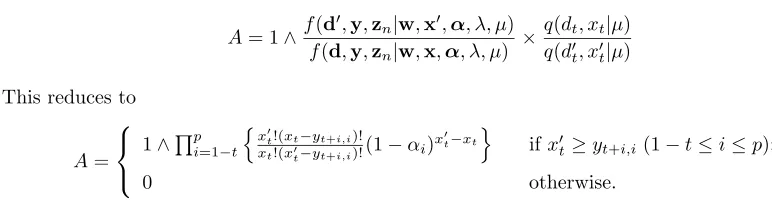
(iii) Calculate the acceptance probability,A, for the move:

A= 1∧f(d

′

,y,zn|w,x

′

,α, λ, µ)

f(d,y,zn|w,x,α, λ, µ)

×q(dt, xt|µ)

q(d′

t, x

′

t|µ)

This reduces to

A=

 



1∧Qp

i=1−_t

n_x′

t!(xt−yt+i,i)!

xt!(x′t−yt+i,i)!(1−αi)

x′

t−xt

o

ifx′

t≥yt+i,i(1−t≤i≤p);

0 otherwise.

Therefore if the move is accepted, set (xt, dt) equal to (x′t, d

′

t), otherwise leave (xt, dt) unchanged.

3. Update µ: Sampleµfrom its conditional distribution given by (3.8).

Then obtaining samples from the posterior predictive distributions ofWpred

m = (Wn+1, Wn+2, . . . , Wn+m)

orXpred

m or both is straightforward, and involves adding the following step to the above MCMC algorithm.

4. Update (xpred_m ,w_mpred): One pair of components at a time, sequentially from (xn+1, wn+1) through

to (xn+m, wn+m). Then for 1≤k≤m, drawzn+k ∼P o(λ),yn+k,i ∼Bin(xn+k−_i, α_i) (1≤i≤p)

anddn+k∼P o(µ). Finally, set

(xn+k, wn+k) =

Ã

zn+k+ p

X

i=1

yn+k,i, zn+k+ p

X

i=1

yn+k,i+dn+k

!

.

4

Results

4.1

Simulation study

In order to assess the strengths and weaknesses of the MCMC algorithms outlined in Section 3, we

conducted an extensive simulation study. A representative sample from the simulation study is given in

Table 1 along with the true model parameters.

Model n α β λ Noise

AR(3) 500 (0.2,0.3,0.15) − 2 −

M A(3) 500 − (0.2,0.3,0.15) 2 −

ARM A(2,2) 500 (0.4,0.2) (0.4,0.2) 2 −

AR(3) + Noise 500 (0.2,0.3,0.15) − 2 P o(1)

For each data set, the MCMC algorithm was run to obtain a sample of size 1000000 following a burn-in

period of 10000 iterations. The burn-in period is essential to ensure that the estimates of the posterior

distribution are unaffected by the choice of starting values of the Markov chain. The priors were chosen

as outlined in Section 3, withπ(λ)∼Gam(1,1) andπ(µ)∼Gam(1,1).

MCMC methods generate dependent samples from the posterior distribution of interest. Therefore it

is essential that a large enough sample is obtained to offset the loss in information (when compared

with an independent and identically distributed sample from the posterior distribution) due to having

a dependent sample. Formal investigation of the performance of the MCMC algorithms, if so desired,

can be done using the integrated autocorrelation function or variance of batch means, see Geyer (1992)

for details. However, visual inspection of the time series plots of the MCMC sample is usually sufficient

to detect that the Markov chain is sampling from its stationary distribution (the posterior distribution).

Also the time series plots allow us to determine how well the Markov chain ismixing, with better mixing

corresponding to less dependence between successive observations of the posterior distribution, and hence,

reduced Monte Carlo error. In Figure 1, time series plots of the first 10000 observations for λfrom the

MCMC sample for each of the four data sets are plotted.

INAR(3)

Observation

lambda

0 2000 6000 10000

1.5

2.0

2.5

3.0

INARMA(2,2)

Observation

lambda

0 2000 6000 10000

1.0

1.5

2.0

2.5

INMA(3)

Observation

lambda

0 2000 6000 10000

1.6

2.0

2.4

INAR(3)+ Noise

Observation

lambda

0 2000 6000 10000

1.0

2.0

3.0

Figure 1. Time series plots for the first 10000 observations ofλ, for theIN AR(3),IN M A(3),

IN ARM A(2,2) and IN AR(3) + N oisedata sets, respectively.

performance with respect to the other parameters. The algorithms are shown to perform well for the INAR

and INMA data sets and not so well for the INARMA and INAR + Noise data sets. The performance of

the MCMC algorithm is closely related to the information content contained within the data about the

various parameters. That is, the more informative the data are about the underlying model parameters,

the better the MCMC algorithms performs. Thus the MCMC algorithm performs very well for INAR(p)

processes since the data (x1−_p, x2−_p, . . . , x_n) is very informative about the parameters driving the process.

However, the MCMC algorithm performs as well for the INMA(q) process (or even better in the above

example) since although the key underlying process (z1−q, z2−q, . . . , zn) is unobserved and needs to be

imputed, the data is very informative about (z1−_q, z₂−_q, . . . , z_n). This is most clearly seen in Table 2

below which lists the estimated mean and standard deviations of the posterior distributions based on the

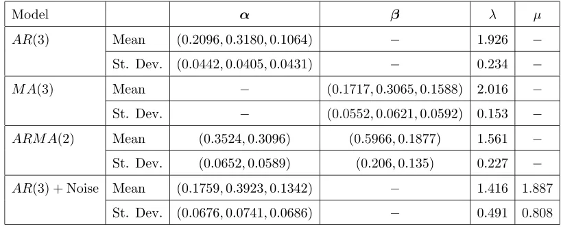
samples obtained from the MCMC algorithms.

Model α β λ µ

AR(3) Mean (0.2096,0.3180,0.1064) − 1.926 −

St. Dev. (0.0442,0.0405,0.0431) − 0.234 −

M A(3) Mean − (0.1717,0.3065,0.1588) 2.016 −

St. Dev. − (0.0552,0.0621,0.0592) 0.153 −

ARM A(2) Mean (0.3524,0.3096) (0.5966,0.1877) 1.561 −

St. Dev. (0.0652,0.0589) (0.206,0.135) 0.227 −

AR(3) + Noise Mean (0.1759,0.3923,0.1342) − 1.416 1.887

St. Dev. (0.0676,0.0741,0.0686) − 0.491 0.808

Table 2. Estimated mean and standard deviations of parameter posterior distributions.

For the INARMA(2,2) data set, the data are more informative about the AR parameters than the MA

parameters. This is generally the case observed for INARMA(p, q) data sets. This is clearly seen in

the estimated variances of the parameter posterior distributions and also by observing the mixing of the

Markov chain for the AR and MA parameters.

The presence of a noise parameter also affects the MCMC algorithm as one would expect. As in Section

3.3, we have restricted attention to INAR(p) processes with noise. Although the noise and signal processes

are independent, the joint posterior distributions for the parameters of the two processes are dependent.

Therefore the stronger the noise is, the harder it is to detect the parameters of the signal (underlying

4.2

Real life data

The main purpose for introducing the MCMC algorithms in Section 3 was to apply the methodology to

real life data. In this section, we apply the methodology of Section 3 to two real life examples Westgren’s

gold particle data set, see Westgren (1916) and Jung and Tremayne (2006) and a Schizophrenic patients

test scores, see McCleary and Hay (1980).

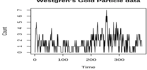
4.2.1 Westgren’s Gold Particle data set

This data set consists of 380 counts of gold particles in a solution at equidistant points in time. The data

was originally published in Westgren (1916) but has recently been analysed in Jung and Tremayne (2006)

using method of moments estimation of an INAR(2) model. Jung and Tremayne (2006) claim that the

INAR(2) is an adequate model for this data basing their analysis on the first 370 observations with the

remaining 10 observations used for predictive purposes. Recent extensions of this paper incorporating

order determination into the MCMC algorithm suggest that the INAR(2) model is indeed the most

suitable INAR model for this data, see Enciso-Moraet al. (2006) for more details.

Westgren’s Gold Particle data

Time

Count

0 100 200 300

0

1

2

3

4

5

6

7

Figure 2. Westgren’s gold particle data set.

Our aim here is to compare our approach with Jung and Tremayne (2006). In particular, we fit an

INAR(2) model to the first 370 observations and estimate the model parameters for the INAR(2) model.

We then obtain the (joint-)predictive distribution for the remaining 10 observations. In Jung and

Tremayne (2006) two INAR(2) models are considered; these are the INAR(2)-AA model (Alzaid and

Al-Osh (1990)) and INAR(2)-DL model (Du and Li (1991)). We have focussed upon the Du and Li

The MCMC algorithm was run in order to obtain samples of size 50000 from the posterior parameter

distribution with a burn-in period of 10000 iterations. These samples were then used to simulate 50000

realisations of the data points 371,372, . . . ,380. The estimated posterior means and standard deviations

for the model parameters are given in the table below. These results are comparable with the parameter

estimates and bootstrap standard errors obtained in Jung and Tremayne (2006).

Parameter α1 α2 λ

Mean 0.463 0.187 0.550

St. dev. 0.0475 0.0540 0.0719

Table 3. Estimates of INAR(2) parameters for Westgren’s data set.

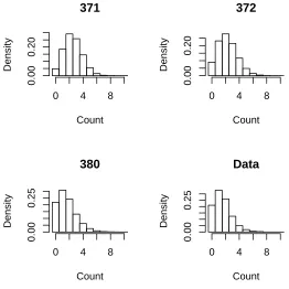
For the (joint-)predictive distribution of the last 10 data points, we obtained identical results to Jung

and Tremayne (2006) for the median predicted values. Below are histograms of the estimated posterior

densities of data points 371, 372 and 380 along with a histogram of the empirical distribution of Westgren’s

data. It is worth noting the close agreement between the predictive distribution for data point 380 and

the empirical distribution of the observed data.

371

Count

Density

0 4 8

0.00

0.20

380

Count

Density

0 4 8

0.00

0.25

372

Count

Density

0 4 8

0.00

0.20

Data

Count

Density

0 4 8

0.00

0.25

Figure 3. Histograms of predictive distributions of data points 371, 372 and 380 and the empirical

4.2.2 Schizophrenic patient

The second example concerns the daily observations of the score achieved by a schizophrenic patient

on a test of perceptual speed, see, McCleary and Hay (1980). The data consists of 120 consecutive

daily scores. However, from the 61st _{day onwards the patient began receiving a powerful tranquilizer}

(chloropromazine) that could be expected to reduce perceptual speed. The data are presented in Figure

4.

Schizophrenic patients’ Test scores

Day

Score

0 20 40 60 80 100 120

30

40

50

60

70

80

90

Figure 4. A time-series plot of the daily test score achieved by schizophrenic patient.

The data clearly shows a reduction in the patients’ test score after day 61. Therefore we propose to

model the patients’ test score using an INAR(1) process with different parameters (α1, λ) for before and

after receiving chloropromazine. Thus the model we used is:

Xt=

 



αB

1 ◦Xt−1+Zt ift≤60

αA

1 ◦Xt−1+Zt ift≥61

whereZt(1≤t≤120) are independent and fort≤60,Zt∼P o(λB) and fort≥61,Zt∼P o(λA). Thus

B andAdenotebeforeandaftertreatment, respectively.

Adapting the likelihood and consequently the MCMC algorithm in Section 3 to incorporate a change

point where the parameter values change is trivial especially in this example where the change point is

known. However, the methodology could also be extended to situations where the position and number

of change points is unknown.

The MCMC algorithm was run in order to obtain samples of size 50000 from the posterior parameter

distribution with a burn-in period of 10000 iterations. The main aim in this example is to study the

affects of chloropromazine on the parameters (α1, λ), however, the posterior predictive distribution can

The samples fromαB1 and αA1 produced indistinguishable posterior density plots. Thus suggesting that

the parameterα1is unaffected by the introduction of treatment and that the data should be modelled with

αB

1 =αA1 =α1. Therefore the MCMC algorithm was run as before except that a common,α1parameter,

for both before and after treatment was used. Posterior density plots for the model parameters from the

two algorithms are given in Figure 5.

0.35 0.45 0.55 0.65

0

2

4

6

8

10

12

14

alpha_1

alpha_1

Density

0 10 30

0.00

0.05

0.10

0.15

0.20

0.25

0.30

lambda

lambda

Density

Figure 5. Posterior density plots for the INAR(1) parameters for the test score, before treatment (solid

lines) and after treatment (dashed lines) in the case (αA

1 6=αB1) and the corresponding parameters

(dotted lines) in the case (αA

1 =αB1 =α1).

The two MCMC algorithms produce indistinguishable results in terms of posterior means forα1,λB and

λA_{. Since a common α}

1 parameter can be assumed, the reduction in test scores is therefore accounted

for by a reduction in theλparameter. The posterior means ofλB_andλA_{are 34.7 (34.8) and 19.2 (19.3),}

respectively, when a commonα1 parameter is used (αB1 6=αA1).

Note that the posterior distribution forα1(α1=αA1 =αB1) is more compact than the individual posterior

distributions for αB

1 and αA1 (αA1 6=αB1). This is since inference for α1 is based on time-series data of

length 120 whereas inference forαB

1 andαA1 time-series data of length 60. This has a knock-on effect of

producing more compact (and peaked) posterior distributions forλB _andλA_{in the case of a commonα}

1

parameter.

5

Conclusions

This paper has introduced an efficient MCMC mechanism for conducting inference for INARMA(p, q)

be very tricky using conventional methods but are very straightforward using MCMC. The methodology

introduced here, as previously mentioned, can readily be extended to incorporate noise, change points

and more general, generalised Steutal and van Harn operators. Thus as a consequence this paper only

scratches the surface of the potential applications of MCMC to integer valued time-series.

Some very natural extensions of the current work present themselves. Firstly, developing inference for

INARMA(p, q) processes where the parameters p and q are unknown. This is the subject of ongoing

research where a reversible jump (RJ) MCMC algorithm has successfully been constructed, see

Enciso-Mora et al. (2006) for details. RJMCMC could also prove useful in extensions of Section 4.2.2 where

both the number and location of parameter change points are unknown. Throughout this paper we have

assumed that the time-series under consideration is stationary. However, this is not necessary for the

above methodology and we could easily adapt the MCMC algorithm to allow for, for example, seasonality

or a linear trend. Finally it would be interesting to study multivariate INARMA(p, q) processes. This

should be, in principle at least, a fairly straightforward extension of the MCMC algorithms in Section 3.

All these extensions should be fairly routine using MCMC algorithms but would prove extremely difficult

problems to tackle using more conventional methods.

Acknowledgements

We thank Robert Jung for providing us with Westgren’s gold particle data set. The schizophrenic patient

data set was obtained from the Time Series Data Library:

http://www-personal.buseco.monash.edu.au/∼hyndman/TSDL/

References

Daniels_{, M. J. and}Cressie_{, N. (2001) A hierarchical approach to Covariance function estimation for}

Time Series. Journal of Time Series Analysis 22, 253–266.

Davis_{, R. A.,} Dunsmuir_{, W. T. M. and} Wang_{, Y. (2000) On autocorrelation in a Poisson regression}

model. Biometrika87, 491–505.

Du_{, J. and}Li_{, Y. (1991) The integer-valued autoregressive (INAR(p)) model. Journal of Time Series}

Enciso-Mora_{, V.,} Neal_{, P. and} Subba Rao_{, T. (2006) Order determination and model selection for}

INARMA(p, q) processes. In preparation.

Franke_{, J. and}Seligmann_{, T. (1993) Conditional maximum likelihood estimates for INAR(1) processes}

and their application to modelling epileptic seizure counts. Time Series Analysis. (ed. T. Subba Rao.)

Chapman and Hall. pp. 310–330.

Freeland_{, R. K. and} McCabe_{, B. P. M. (2004) Forecasting discrete valued low count time series.}

International Journal of Forecasting20, 427–434.

Geyer_{, C.J. (1992) Practical Markov chain Monte Carlo (with discussion).} Statistical Science7, 473–511.

Gilks_{, W. R.,}Richardson_{, S. and}Spiegelhalter_{, D. J. (eds.) (1995)Markov chain Monte Carlo in}

Practice. Chapman and Hall.

Jung_{, R. C. and Tremayne, A. R. (2006) Coherent forecasting in integer time series models. International}

Journal of Forecasting22, 223–238.

Latour_{, A. (1997) The multivariate GINAR(p) process. Advances in Applied Probability29, 228–248.}

McCabe_{, B. P. M. and}Martin_{, G. M. (2005) Bayesian predictions of low count time series. International}

Journal of Forecasting22, 315–330.

McCleary_{, R. and} Hay_{, R. A. (1980) Applied Time Series Analysis for the Social Sciences. Sage}

Publications.

McKenzie_{, E. (2003) Discrete variate time series. Stochastic Processes: Modelling and Simulation. (eds.}

D. N. Shanbhag and C. R. Rao.) Elsevier. pp. 573–606.

Steutel_{, F. W. and} van Harn_{, K. (1979) Discrete analogues of self-decomposability and stability.}

Annals of Probability7, 893–899.

Troughton_{, P. T. and} Godsill_{, S. J. (1997) Bayesian model selection for time series using Markov}

chain Monte Carlo. InProc. IEEE International Conference on Acoustics, Speech and Signal Processing

1997, vol. V.3733–3736.

Westgren_{, A. (1916). Die Ver¨anderungsgeschwindigkeit der lokalen Teilchenkonzentration in kollioden}