Munich Personal RePEc Archive
Adversarial scheduling analysis of
Game-Theoretic Models of Norm
Diffusion.
Istrate, Gabriel and Marathe, Madhav V. and Ravi, S.S.
e-Austria Research Institute
9 April 2008
Online at
https://mpra.ub.uni-muenchen.de/8170/
Adversarial Scheduling Analysis of
Game-Theoretic Models of Norm Diffusion
Gabriel Istrate1⋆, Madhav V. Marathe2, and S.S. Ravi3
1
e-Austria Institute, V.Pˆarvan 4, cam. 045B, Timi¸soara RO-300223, Romania
2 Network Dynamics and Simulation Science Laboratory, Virginia Tech, 1880 Pratt
Drive Building XV, Blacksburg, VA 24061. Email:[email protected]
3 Computer Science Dept., S.U.N.Y. at Albany, Albany, NY 12222, U.S.A.
Email:[email protected]
Abstract. In [IMR01] we advocated the investigation of robustness of results in the theory of learning in games under adversarial scheduling models. We provide evidence that such an analysis is feasible and can lead to nontrivial results by investigating, in an adversarial scheduling setting, Peyton Young’s model of diffusion of norms [You98]. In particular, our main result incorporatescontagioninto Peyton Young’s model.
Keywords:evolutionary games, adversarial scheduling, discrete Markov chains.
1
Introduction
Game-theoretic equilibria aresteady-state properties; that is, given that all the players’ actions correspond to an equilibrium point it would be irrational for any of them to deviate from this behavior when the others stick to their strategy. The fundamental problem facing this type of concept is that it does not predict
how players arrive at this equilibrium in the first place, or how they “choose” one such equilibrium, if several such points exist. The theory of equilibrium selection of Hars´anyi and Selten [HS88] assumes some form of prior coordination between players, in the form of a tracing procedure. This strong prerequisite is often unrealistic.
The theory oflearning in games[FL99] attempts to explain the emergence of equilibria as the result of an evolutionary “learning” process. Models of this type assume one (or several) populations ofagents, that interact by playing a certain game, and updating their behavior based on the outcome of this interaction.
Results in evolutionary game theory are important not necessarily as realis-tic models of strategic behavior. Rather, they provide possible explanations for experimentally observed features of real-world social dynamics. For instance, the fundamental insight behind the concept ofstochastically stable strategiesis that continuous “noise” (or small deviations from rationality) can provide a solution to the equilibrium selection problem in game theory. discussion on the role of
strategic learning in equilibrium selection see [PY05]) Similar issues apply when mathematical modeling is replaced with computer experiments, in the area of
agent-based social simulation [GT05]. Epstein [Eps07] (see also [AE96]) has ad-vocated a generative approach to social science: in order to better understand a given phenomenon one should be able to generate it via simulations.
Given that such mathematical models or simulations are emerging as tools for policy-making (see e.g. [NBB99,ECC+04]), how can we be sure that the conclusions that we derive from the output of the simulation do not crucially depend on the particular assumptions and features we embed in it ? Part of the answer is that these results have to display “robustness” with respect to the various idealizations inherent in the model, be it mathematical or computational. Various issues that might impact the robustness of the conclusions have been previously considered in the game-theoretic literature; for instance, the cele-brated result of Foster and Young [FY90] can be viewed as investigating the robustness of Nash equilibria with respect to the introduction of small amounts of random noise (or player mistakes).
In this paper we are only concerned with one such issue:scheduling, i.e.the order in which agents get to update their strategies. Two alternatives are most popular, both in the mathematical and the computer simulation literature: in the
synchronous mode (every player updates at every step. A popular alternative is
uniform matching. Models of the latter type assume an underlying (hyper)graph topology (describing the sets of players allowed to simultaneously update in one step as a result of game playing) and choose a (hyper)edge uniformly at random from the available ones. Employing a uniform matching model in mul-tiagent models of social systems is unrealistic for it assumes perfect and global
randomness; it is not clear whether this assumption is waranted in the “real life” situations that the theory is supposed to model. Indeed, notwithstanding the question regarding the existence of computational randomness in nature, the structure of social interactions is neither random, nor uniform, and comprises many regular, “day by day” interactions, as well as a smaller number of “oc-casional” ones. A random matching model does not take into account locality
and cannot, therefore, adequately model “contagion” effects (i.e. players becom-ing activated as a result of some of their neighbors dobecom-ing so) . On the other hand, social systems areinherently distributed, and it is not clear whether the assumption ofglobalrandomness is reasonable in a simulation setting.
that modelscontagionand has a certainreversibilityproperty (the class of such schedulers includes the random scheduler as a special case). However for this class of schedulers theconvergence time isnotnecessarily the one from the case of random scheduling.
Besides the relevance of our results to evolutionary game-theory, we hope that the concepts and techniques relevant to this paper can be fruitfully exploited in the theory of rapidly mixing Markov chains, of great interest in Theoretical Computer Science.
Not surprisingly, our framework is related to thetheory of self-stabilization of distributed systems [Dol00]. Our proofs highlight some principles and tech-niques of this theory (the existence of a winning strategy for scheduler-luck games
[Dol00],monotonicityandcomposition of winning strategies) that can be applied to the particular problem we study, and conceivably in more general settings as well.
2
Preliminaries
A general class of models for which adversarial analysis can be naturally consid-ered is that ofpopulation games[Blu01]. Systems of interest in this class consist of a number ofagents, defined as the vertices of a hypergraphH = (V, E). One edge of this hypergraph represents a particular choice of all players who can play (one or more simultaneous instances of) a game G that defines the dynamics. Each player has astate(generally a mixed strategy ofG) chosen from a certain set S. The global state of the system is an element of S =SV. The dynamics
proceeds by choosing one edge e of H (according to a scheduling mechanism that is specified by the scheduler), letting the agents in e play the game, and updating their states as a result of game playing.
2.1 Schedulers
Denote byX∗ the set of finite words over alphabetX.
Definition 1. Adeterministic scheduleris specified by a mappingf :E∗×S→
E, where E is the set of edges of H and S is the set of possible states of the system. Mappingf specifies the next scheduled element, given the current history. Let b ≥1. A scheduler that can choose one item among a set ofm elements is
(worst-case) b-fair if every agent is guaranteed to be scheduled at least once in any sequence ofb(m−1) + 1consecutive steps.
One particularly restricted class of schedulers is that ofnon-adaptive sched-ulers, corresponding to updates of the nodes/edges according to a fixed permu-tation, independent of the initial state of the system.
The above definitions are well-suited for deterministic schedulers. They are
notwell-suited for probabilistic schedulers (such as random matching), since for any fixed number of stepsB with positive probability it will take more thanB
for multiple agents to be scheduled simultaneously. Therefore in this case we need to employ slightly different definitions.
Definition 2. A(probabilistic) schedulerassigns a probability distributionpw,s
on E to each pair (w, s, s0) consisting of initial prefixes w ∈ E∗, s ∈ S∗ with
|w| = |s| and starting state s0 ∈ S. The next element e ∈ E to be scheduled,
given prefixes w, sand initial states0, is sampled from E according topw,s,s0.
Anon-adaptiveprobabilistic scheduler is specified by (a) a collection (multi-set) Σ={D1, . . . ,Dm} of probability distributions on the set E such that every
x∈E belongs to the support of some distributionDiand (b) a fixed permutation
π of Σ. The scheduler proceeds by (possibly concurrently) scheduling elements of E sampled from a distribution fromΣ chosen according to (consecutive rep-etitions of ) permutation π. For C >0, a non-adaptive probabilistic scheduler is
C individually-fair if for everyx∈E, the probability that xis scheduled during one round of πis at leastC/|E|.
One can define, for any given triple (w, s, s0), where w ∈ E∗, s ∈ S∗ and
s0 ∈ S, a probability πw,s,s0, the probability that, starting from state s0 the
scheduler uses was the initial prefix of its schedule and evolves its global state according to strings. Let Ω denote the resulting probability space. We divide each trajectory of a probabilistic scheduler into rounds: the first round is the smallest initial segment that schedules each element of E at least once, the second round is the smallest segment starting at the end of the first round that schedules each element at least once, and so on. Given this convention, it is easy to see that for any k > 0 ands ∈ S the family Wk of strings w consisting of
exactly k rounds realizes a complete partition of the probability space Ω, i.e.
P
w∈Wkπw,s= 1.
Definition 3. If f(·) is a function on integers, we say that a family of prob-abilistic schedulers, indexed by n, the cardinality of the set E, is O(f(n))-fair w.h.p. if there exists a monotonically decreasing function g : (0,∞) → (0,1), with limǫ→∞g(ǫ) = 0 such that for every state s ∈ S, denoting by li the
ran-dom variable measuring the length of thei’th round, we havelimn→∞Prob[li>
ǫ·f(n)]< g(ǫ).
Random scheduling can be specified by a non-adaptive probabilistic scheduler whose setΣconsists of just one distribution, namely the uniform distribution on
E. This scheduler is 1-individually fair and, by the well-known Coupon Collector Lemma it is alsoO(nlog(n))-fair w.h.p.
2.2 Peyton Young’s model of norm diffusion
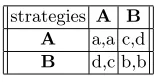
The setup of this model is the following: agents located at the vertices of a graphG interact by playing a two-person symmetric game with payoff matrix
M = (mi,j)i,j∈{A,B} displayed in Figure 1. It is assumed that strategy Ais a
“importance”. When scheduled, agents play (using the same strategy, identified as the agent’s state) against each of their neighbors. If agent i is the one to update,xis the joint profile of agents’ strategies, andz∈ {A,B}is the candidate new state, pβ(x
i →z|x) ∼eβ·νi(z,x−i), where νi(z, x−i), the payoff of thei’th
agent should he play strategy z while the others’ profile remains the same is given byνi(z, x−i) =P(i,j)∈Ewijmz,xj. Under random scheduling, the process
we defined is a variant of the best-response dynamics. This latter process (viewed as a Markov chain) is not ergodic. Indeed, the since in gameGit is always better to play the same strategy as your partner, the dynamics has at least two fixed points, states “allA” and “allB”.
strategies A B A a,a c,d
[image:6.595.267.344.257.298.2]B d,c b,b
Fig. 1.Payoff matrix
An important property of Peyton Young’s dynamics is that it corresponds to apotential game:there exists a functionρ:V →Rsuch that, for any player
i, any possible actions a1, a2 of player i, and any action profile a of the other players,ui(a1, a)−ui(a2, a) =ρ(a1, a)−ρ(a2, a) (whereui is the utility function
of player i). In other words changes in utility as a result of strategy update correspond to changes in a global potential function. An explicit potential is given byρ∗(x) =P
(h,k)∈Ewh,kmxh,xk.
2.3 Stochastic stability
A fundamental concept we are dealing with is that of astochastically stable state
for dynamics described by a Markov chain.
Definition 4. Consider a Markov process P0 defined on a finite state spaceΩ.
For each ǫ > 0, define a Markov process Pǫ on Ω. Pǫ is a regular perturbed
Markov processif all of the following conditions hold.
– Pǫ is irreducible for everyǫ >0.
– For everyx, y∈Ω, limǫ>0Pxyǫ =Pxy0 .
– IfPxy >0 then there existsr(m)>0, theresistance of transitionm= (x→
y), such that as ǫ→0,Pǫ
xy=Θ(ǫr(m)).
Letµǫbe the (unique) stationary distribution ofPǫ. A statesisstochastically
stable iflimǫ→0 µǫ(s)>0.
Observation 1 Peyton Young’s model of diffusion of norms can be recast into the framework of Definition 4. Let ǫ =exp(−β). As β → ∞, ǫ→ 0. Consider now the Markov chain Γǫ corresponding to the original dynamics. It has
tran-sition matrix Dǫ =D1,ǫ. . . Dm,ǫ, where Di,ǫ = (dǫi,k,l) is the transition matrix
corresponding to scheduling (and updating) a node according toDi. It is easy to
see that limǫ→0dǫk,l =dk,l. Moreover, by the nature of the dynamics, as ǫ→0
each element of Di,ǫ is either zero (in case the state transition k → l cannot
be realized by updating any single node member of supp(Di)), tends to a
posi-tive constant which is the probability that the node corresponding to the transition
k→lis chosen (in case the transitionk→lcorresponds to a “best reply” move), or tends to zero, asymptotically like Θ(ǫri,k,l), for somer
i,k,l>0 (otherwise).
Definition 5. A tree rooted at node j is a set T of edges such that for any statew6=j there exists a unique (directed) path from wto j. Theresistance of a rooted treeT is the sum of resistances of all edges inT.
The following characterization of stochastically stable states is presented as Lemma 3.2 in the Appendix of [You98]:
Proposition 6. Let Pǫ be a regular perturbed Markov process, and for each
ǫ > 0 let µǫ be the unique stationary distribution of Pǫ. Then lim
ǫ→0µǫ =µ0
exists, andµ0 is a stationary distribution of P0. The stochastically stable states
are precisely those states z such that there exists a tree rooted at z of minimal resistance (among all rooted trees).
Definition 7. Given a graphG, a nonempty subsetSof vertices and a real num-ber0≤r≤1/2we say thatSisr-close-knitif∀S′⊆S, S′6=∅, e(S′
,S)
P
i∈S′deg(i)≥r,
where e(S′, S)is the number of edges with one endpoint in S′ and the other in
S, and deg(i) is the degree of vertex i. A graph G is (r, k)-close-knit if every vertex is part of ar-close-knit set S, with|S|=k.
Definition 8. Given p ∈ [0,1], the p-inertia of the process is the maximum, over all states x0 ∈ S, of W(β, p, x0), the expected waiting time until at least 1−pof the population is playing actionAconditional on starting in state x0.
The model in [You03,You98] assumes independent individual updates, ar-riving at random times governed (for each agent) by a Poisson arrival process with rate one. Since we are, however, interested in adversarial models that do not have an easy description in continuous time we will assume that the process proceeds in discrete steps. At each such step a random node is scheduled. It is a simple exercise to translate the result in [You03,You98] to an equivalent one for global, discrete-time scheduling. The conclusions of this translation are:
– The stationary distribution of the process isthe Gibbs distribution,µβ(x) = eβρ(x)
P
zeβρ(x), whereρis the potential function of the dynamics.
– ”AllA“ is the unique stochastically-stable state of the dynamics.
3
Results
First we note that Peyton Young’s results easily extend to non-adaptive sched-ulers. Adaptive schedulers on the other hand, even those of fairness no higher than that of the random scheduler, can preclude the system from ever enter-ing a state where a proportion higher thanr of agents plays the risk-dominant strategy:
Theorem 9. The following hold:
(i) Forall non-adaptive schedulers, the state “all A” is the unique stochas-tically stable state of the system.
(ii) LetG be a class of graphs that are(r, k)-close-knit for some fixedr > r∗.
Let f =f(n)be a class of non-adaptiveΘ(1)individually fair schedulers. Given any p∈(0,1) there exists a βp such that for all β > βp there exists a constant
C such that thep-inertia of the process (under scheduling given by f) is at most
C·m·n, wherem=m(n)is the number of rounds of f andnis the number of vertices of the underlying graph.
(iii) For every0< r <1there exists an adaptivescheduler which isO(nlog(n)) -fair w.h.p. (where the constant hidden in the “O” notation depends on r) that can forever prevent the system, started on the “allB’s” configuration, from ever having more than a fraction ofr of the agents playingA.
(i) Leti∈V and letMi be the restriction of the given dynamics corresponding
to the case when only one node, nodei, is scheduled in all moves (otherwise the dynamics is similar to the original one).
It is easy to see that Mi is a non-ergodic Markov chain and that µβ is
a stationary distribution for the Markov chain Mi. This is so because for
two configurationsx, y that only differ in positioni, the ratio of transition probabilitiespx,y/py,xis equal to toexp[β·(ρ∗(x)−ρ∗(y))], which is precisely
µβ(x)/µβ(y).
Now consider the matrixDkcorresponding to the distribution with the same
notation as in the periodic schedule. It is a convex combination of the ma-tricesMi, hence it will also haveµβ as a stationary distribution. We infer
that the product of matricesDk corresponding to the cyclic schedule also
hasµβ as a stationary distribution.
But it is easy to see that the Markov chain corresponding to one round of the cyclic schedule is irreducible (since one can navigate between any two states in at most|V| rounds, by flipping the differing bits and keeping the bits that coincide fixed) and aperiodic (since the probability of remaining in a given state is positive). Therefore, it must have an unique stationary distribution, which is necessarilyµβ.
(ii) Consider a vertex v ∈ V and a r-close-knit set of size k containing v, de-notedSv. ConsiderΓv,β the version of the process where each vertex in Sv
updates just as before, but each vertex in V \Sv always chooses state B
This restricted dynamics onV still corresponds to a potential game, specified by potential function
ρ∗(x) = X (i,j)∈E
ρ(xi, xj), forx∈ {A, B}SvBV\Sv,
and with the Gibbs distribution µβ(x) = eβ·ρ∗(x) P
zeβ·ρ
∗(z) as its stationary
dis-tribution. Again, just as in [You93] (since the precise scheduling order does
notplay a role in this result) the condition thatGis (r, k)-close-knit implies that the stateAS defined as “allA” onSv and “allB” onV\Svis the state
with the highest potential among the possible states of the system.
One additional complication of the dynamicsΓv,β is that it often schedules
(unnecessarily) nodes outsideSv, that do not change. ConsiderΞv,βthat is
the version ofΓv,β that “only schedules nodes in Sv” (i.e. it ignores moves
ofΓv,β that schedule nodes outside ofSv).
To describe this dynamics formally, view each distribution Di as a set of
symbols from the alphabetV. Then the set of trajectories of the dynamics
Γv,βcan be specified by the words of the regular languageLΓ = (D1·D2·. . .·
Dm)∗. Trajectories ofΞv,βcorrespond to words in another regular language
LΞ, more precisely to the ones corresponding to deleting symbols inV \Sv
from words in LΓ. This regular language can be specified by the regular
expression ((D1∪ {λ})·. . .·(Dm∪ {λ})∩Sv+)∗. This expression yields a
matrix of size 2|Sv|×2|Sv|forΞ
v,β.
Claim. For everyǫ >0 there existsη ∈Nsuch that, for every η′ > η ∈N
any initial state ofΓv,β and every stateT ∈ {A,B}Sv.
|P r[Γv,β in stateT | |w|=η′·m·n]−Π(T)| ≤ǫ.
Proof. Let ǫ > 0. As Ξv,β converges to its stationary distribution, there
existsk >0 such that∀k′> k and every initial state of Ξv,β
|P r[Ξv,β in stateT||w|=k′]−Π˜(T)| ≤ǫ/2, (1)
where ˜Π is the stationary distribution of dynamicsΞ. Of course, states with positive support in ˜Π have the same probability inΠ, that is
∀T ∈ {A,B}Sv: Π(T) = ˜Π(v).
Let Y be a random trajectory of length η′ ·m·n in l
Γ and let pr(Y) its
projection ontoLΞ.
Claim. There existsη >0 such that∀η′> η
Prob
|Y|=η′·m·n[|pr(Y)|< k]≤
ǫ
Proof. The probability that any given distribution Di whose support
in-cludes some element inSvwill schedule (in a given round) a node in this set
isΩ(1/n), by the fairness condition. There is at least one suchDi among all
them distributions. Therefore, the expected length ofpr(Y) isΩ(k/n). A simple application of Markov’s inequality gives the desired result.
Now write
P r [Γv,β in stateT||w|=η′·m·n]
=Pj P r[Γv,β in stateT | |w|=η′·m·n,|pr(w)|=j]
· Prob[|pr(w)|=j]
Therefore we have
P r [Γv,β in stateT||w|=η′·m·n]−Π(t)| ≤
≤Pj|P r[Γv,β in stateT | |w|=η′·m·n,|pr(w)|=j]−Π(T)| ·
· Prob[|pr(w)|=j]
The first term in the product is an absolute difference between two probabil-ity values, and thus has absolute value at most one. Therefore, by Claim ii, if we neglect in the sum those terms withj < konly changes the sum by at mostǫ/2. On the other hand
P r[Γv,β in stateT | |w|=η′·m·n,|pr(w)|=j]
=P r[Ξv,β in stateT||w|=k′].
Now, using Equation (1), Claim ii follows.
From now on the proof mirrors rather closely the one for the case of ran-dom scheduling (presented in the Appendix to [You93]): first, because the stationary distribution of processΓ is the Gibbs distribution, there exists a finite valueβ(Γ, S, p) such thatµv(AS)≥1−p2/2 for allβ > β(Γ, S, p).
There are only a finite number of nonisomorphic dynamical systems Γv,β
(where isomorphism of dynamical system is meant to be the isomorphism of the underlying graph topologiesSv and of the projection of schedulers onto
Sv). In particular we can findβ(r, k, p) andη(r, k, p) such that, for all graphs
G∈ G and all r-close-knit subsets S withk vertices, the following relation holds forallinitial states:
∀β ≥β(r, k, p),∀η′ ≥η, P r[yη′
·m·n =A
S]≥1−p2. (2)
whereyt is the state of the dynamical system on stateS
v at timet. We can
now derive that for every close-knit setS
∀β≥β(r, k, p),∀η′ ≥η, P r[xη′
·m·n=A
where xt is now the state of the process from the theorem. The argument
is obtained via essentially the same coupling as the one from [You98], hence it is omitted from this writeup. Since every vertexiis contained in a (r, k )-close-knit set, it follows that
∀β ≥β(r, k, p),∀η′≥η, P r[xiη′·m·n=A]≥1−p2.
Therefore the expected proportion of vertices playing actionAat timeη′·m·n
is at least (1−p2)n. But this implies that
∀t≥η·m·n, P r[ at least (1−p)nnodes have labelA]≥1−p.
Indeed, if this wasn’t the case, then with probability at leastpmore thanpn
nodes at timetwould have labelB, a contradiction. Now, by an application of Markov’s inequality, the expected time until at least (1−p)nnodes are labelledAis at mostη·m·n/(1−p). Since this holds for all graphsGinG, thep-inertia of the process is bounded as stated in the theorem.
(iii) Consider a scheduler working in rounds. In each round the scheduler is scheduling nodes according to a fixed permutationπ, the same for all rounds. In each round the scheduler is scheduling each node at least once. For the first⌈rn⌉+ 1 nodes the scheduler continues scheduling each of them (after the initial one) until the node switches to strategyB. The scheduler plays each remaining nodeexactlyonce.
It is easy to see that there exists a constantǫ >0 (that may depend onβ) such that, at each stage, each agent switches to strategyBwith probability greater or equal toǫ.
Therefore the probability that any given agent needs to be scheduled for more thanclog(n) rounds before turning toBis o(1/n) for large enoughc. It follows that the given scheduler isO(nlog(n))-fair w.h.p.
3.1 Main result: Diffusion of norms by contagion
Adaptive schedulers can display two very different notions of adaptiveness:
(i) The next node depends only on the set of previously scheduled nodes, or (ii) It crucially depends on thestatesof the system so far.
The adaptive schedulers in Theorem 9 (iii) was crucially using the second, stronger, kind of adaptiveness. In the sequel we study a model that displays adaptiveness of type (1) but not of type (2). The model is specified as follows: To each node v we associate a probability distribution Dv on the vertices of
G. We then choose the next scheduled node according to the following process. If ti is the node scheduled at stage i, we choseti+1, the next scheduled node,
by sampling from Dti. In other words, the scheduled node performs a
case that v ∈ supp(Dv). Also, let H be the directed graph with edges defined
as follows: (x, y) ∈ E[H] ⇐⇒ (y ∈ supp(Dx)). This dynamics generalizes
both the class of non-adaptive schedulers from previous result and the random scheduler (for the case when H is the complete graph). In the context of van Rooy’s evolutionary analysis of signalling games in natural language [Roo04], it functions as a simplified model for an essential aspect of emergence of linguistic conventions: transmission viacontagion.
It is easy to see that the dynamics can be described by an aperiodic Markov chainM on the set onV{A,B}×V, where a state (w, x) is described as follows:
– wis the set of strategies chosen by the agents.
– xis the label of the last agent that was given the chance to update its state. If the directed graphH is strongly connected then the Markov chain M is irreducible, hence it has a stationary distribution Π. We will, therefore, limit ourselves in the sequel to settings with strongly connectedH. We will, further, assume that the dynamics isweakly reversible, i.e. (x∈supp(Dy)) if and only if
(y∈supp(Dx)). This, of course, means that the graphHis undirected. Note that
since we do not constrain otherwise the transition probabilities of distributions
Di, the stationary distribution Π of the Markov chain doesnot, in general,
de-compose as a product of component distributions. That is, one cannot generally writeΠ(w, x) asΠ(w, x) =π(w)·ρ(x), for some distributionsπ, ρ.
Theorem 10. The setQ={(w, x)|w=VA} is the set of stochastically stable
states for the diffusion of norms by contagion.
Proof. The states inQare obviously reachable from one another by zero-resistance moves, so it is enough to consider one statey ∈Qand prove that it is stochas-tically stable. To do so, by Proposition 6, all we need to do is show thatyis the root of a tree of minimal resistance. Indeed, consider another state x∈Q and letT be a minimum potential tree rooted atx.
Claim. There exists a treeT rooted at y having potential less or equal to the potential of the tree T, strictly smaller in case x is not a state having all its first-component labels equal toA.
Let πy,x = (x0, i0) → (x1, i1) → . . . → (xk, ik) → (xk+1, ik+1) → . . . →
(xr, ir) be the path fromyto xin T (that is (x0, i0) =y, (xr, ir) =x).
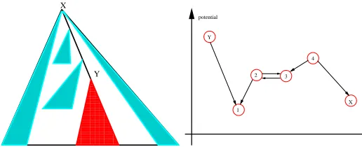
We will defineT by viewing the set of edges ofT as partitioned into subsets of edges corresponding to paths as follows (see Figure 2 (a)):
(i) The set of edges of pathπy,x.
(ii) The set of edges of the subtree rooted aty.
(iii) Edges of tree components (perhaps consisting of a single node) rooted at a node ofπy,x, other thany (but possibly beingx).
0000000000 0000000000 0000000000 0000000000 0000000000 0000000000 0000000000 0000000000 0000000000 0000000000 0000000000 0000000000 0000000000 0000000000 0000000000 0000000000 0000000000 0000000000 0000000000 0000000000 0000000000 0000000000 0000000000 0000000000 0000000000 0000000000 0000000000 0000000000 0000000000 1111111111 1111111111 1111111111 1111111111 1111111111 1111111111 1111111111 1111111111 1111111111 1111111111 1111111111 1111111111 1111111111 1111111111 1111111111 1111111111 1111111111 1111111111 1111111111 1111111111 1111111111 1111111111 1111111111 1111111111 1111111111 1111111111 1111111111 1111111111 1111111111 X Y Y X potential 4 3 2 1
Fig. 2.(a). Decomposition of edges of treeT (b). Resistance of edges on a path between two nodesX andY.
(i) Instead of path πy,x we add path Πx,y from x to y defined by: Πx,y =
(xr, ir)→(xr−1, ir)→(xr−2, ir−1)→. . .→(x0, i1)→(x0, i0) =y. (ii) Rooted trees of type (2) are included into treeT as well.
(iii) The transformation is more complicated for the third type of edges, and we explain it in detail. LetWk be a tree component of T, connected to path
πy,xat connection point (xk, ik).
Case 1: xk =xk−1. Then the point (xk, ik) = (xk−1, ik) belongs to path
Πx,y as well, so one can just add the rooted tree Wk toT as well.
Case 2: xk 6=xk−1 and the move (xk−1, ik−1) → (xk, ik) has positive
re-sistance. In this case, since in configurationxk−1 and scheduled nodeik we
have a choice of either moving toxk or staying in xk−1, it follows that the
move (xk, ik)→(xk−1, ik) has zero resistance.
Therefore we can add toT the treeWk =Wk∪ {(xk, ik)→(xk−1, ik)}. The
tree has the same resistance as the one of treeWk.
Case 3:xk−16=xk and the move (xk−1, ik−1)→(xk, ik) has zero resistance.
Letj be the smallest integer such that either xk+j+1 =xk+j or xk+j+1 6=
xk+j and the move (xk+j, ik+j)→(xk+j+1, ik+j+1) has positive resistance.
In this case, one can first replace Wk by Wk ∪ {(xk, ik) → (xk+1, ik+1),
(xk+1, ik+1) → . . . → (xk+j, ik+j)} without increasing its total resistance.
Then we apply one of the techniques from Case 1 or Case 2.
Case 4:xk−1 6= xk, the move (xk−1, ik−1)→ (xk, ik) has zero resistance,
and all moves on πy,x, from xk up to x have zero resistance. Then define
Wk=Wk∪(xk, ik)→(xk+1, ik+1)→. . .→x.
It is easy to see that no two sets Wk intersect on an edge having positive
resistance. The union of the paths of all the sets is a directed associated graphW
rooted aty, that contains a rooted treeTof potential no larger than the potential of W. Since transformations in cases (i),(iii) do not increase tree resistance, to compare the potentials of T and W it is enough to compare the resistances of pathsπy,x andΠx,y.
values of the potential function at three points:a1, a2anda3, wherea3is the state obtained by assigning nodej2the value not assigned by move toa2. Specifically,
r(m)>0 if either ρ∗(a2)< ρ∗(a1), in which caser(m) =ρ∗(a1)−ρ∗(a2), or
a2 =a1 and ρ∗(a3)> ρ∗(a1), in which case r(m) = ρ∗(a3)−ρ∗(a1). In other words, the resistance of a move is positive in the following two cases: (1) The move leads to a decrease of the value of the potential function. In this case the resistance is equal to the difference of potentials. (2) The move corresponds to keeping the current state (thus not modifying the value of the potential function), but the alternate move would have increased the potential. In this case the resistance is equal to the value of this increase.
Let us now compare the resistances of pathsπy,x and Πx,y. First, the two
paths contain no edges of infinite resistance, since they correspond to possible moves under Markov chain dynamicsPǫ. If we discount second components, the
two paths correspond to a single sequence of statesZ connectingx0toxr, more
precisely totraversingZ in opposite directions. (The last move inΠx,y has zero
resistance and can thus be discounted). Resistant moves of type (2) are taken into account by both traversals, and contribute the same resistance value to both paths. So, to compare the resistances of the two paths it is enough to compare resistance of moves of type (1). Moves of type (1) of positive resistance are those that lead to a decrease in the potential function. Decreasing potential in one direction corresponds to increasing it in the other (therefore such moves have zero resistance in the opposite direction).
An illustration of the two types of moves is given in Figure 2 (b), where the path between X andY goes through four other nodes, labeled 1 to 4. The relative height of each node corresponds to the value of the potential function at that node. Nodes 2 and 3 have equal potential, so the transition between 2 and 3 contributes an equal amount to the resistance of paths in both directions (which may be positive or not). Other than that only transitions of positive resistance are pictured.
The conclusion of this argument is thatr(πy,x)−r(Πx,y) =ρ∗(x)−ρ∗(y)≥0,
andr(πy,x)−r(Πx,y)>0 unlessxis an “allA” state.
3.2 The inertia of diffusion of norms with contagion
Theorem 10 shows that random scheduling is not essential in ensuring that stochastically stable states in Peyton Young’s model correspond to all players playing A: the same result holds in the model with contagion. On the other hand, the result on thep-inertia of the process on families of close-knit graphs is
In the journal version of the paper we will present an upper bound on the
p-inertia for the diffusion of norms with contagion based on concepts similar to theblanket timeof a random walk [WZ96].
4
Conclusions and Acknowledgments
Our results have made the original statement by Peyton Young more robust, and have highlighted the (lack of) importance of various properties of the random scheduler in the results from [You98]: thereversibility of the random scheduler, as well as its inability to use the global system state are important in an adver-sarial setting, while its fairness properties are not crucial for convergence, only influencing convergence time. Also, the fact that the stationary distribution of the perturbed process is the Gibbs distribution (true for the random scheduler) does not necessarily extend to the adversarial setting.
This work has been supported by the Romanian CNCSIS under a PN-II “Idei” Grant, by the U.S. Department of Energy under contract W-705-ENG-36 and by NSF Grant CCR-97-34936.
References
[AE96] R. Axtell and J. Epstein. Growing Artificial Societies: Social Science from the Bottom Up. The MIT Press, 1996.
[Blu01] L. Blume. Population games. In S. Durlauf and H. Peyton Young, editors,
Social Dynamics: Economic Learning and Social Evolution. MIT Press, 2001. [Dol00] S. Dolev. Self-stabilization. M.I.T. Press, 2000.
[ECC+
04] J.M. Epstein, D. Cummings, S. Chakravarty, R. Singa, and D. Burke. To-ward a Containment Strategy for Smallpox Bioterror. An Individual-Based Computational Approach. Brookings Institution Press, 2004.
[Eps07] J. Epstein.Generative Social Science: Studies in Agent-based Computational Modeling. Princeton University Press, 2007.
[FL99] D. Fudenberg and D. K. Levine. The Theory of Learning in Games. M.I.T. Press, 1999.
[FY90] D. Foster and H .P. Young. Stochastic evolutionary game dynamics. Theo-retical Population Biology, 38(2):219–232, 1990.
[GT05] N. Gilbert and K. Troizch. Simulation for social scientists (second edition). Open University Press, 2005.
[HS88] J. Hars´anyi and R. Selten. A General Theory of Equilibrium Selection in Games. The M.I.T. Press, 1988.
[IMR01] G. Istrate, M.V. Marathe, and S.S. Ravi. Adversarial models in evolution-ary game dynamics. InProceedings of the 13th ACM-SIAM Symposium on Discrete Algorithms (SODA’01), 2001. (journal version in preparation). [NBB99] K. Nagel, R. Beckmann, and C. Barrett. TRANSIMS for transportation
planning. In Y. Bar-Yam and A. Minai, editors,Proceedings of the Second International Conference on Complex Systems. Westview Press, 1999. [PY05] H. Peyton-Young. Strategic Learning and Its Limits. Oxford University
[Roo04] R. Van Rooy. Signalling games select Horn strategies. Linguistics and Phi-losophy, 27:423–497, 2004.
[WZ96] P. Winkler and D. Zuckerman. Multiple cover time.Random Structures and Algorithms, 9(4):403–411, 1996.
[You93] H.P. Young. The evolution of conventions.Econometrica, 61(1):57–84, 1993. [You98] H.P. Young.Individual Strategy and Social Structure: an Evolutionary
The-ory of Institutions. Princeton University Press, 1998.