Inference of systems with delay and applications to cardiovascular dynamics

c

World Scientific Publishing Company

INFERENCE OF SYSTEMS WITH DELAY

AND APPLICATIONS TO CARDIOVASCULAR DYNAMICS

A. BANDRIVSKYY, D .G. LUCHINSKY, P. V. E. McCLINTOCK

Department of Physics, Lancaster University, Lancaster, LA1 4YB, UK. [email protected], [email protected], [email protected]

V. N. SMELYANSKIY

NASA Ames Research Center, MS 269-2, Moffett Field, CA 94035-1000, USA. [email protected]

A. STEFANOVSKA

Nonlinear Dynamics and Synergetics, Faculty of Electrical Engineering, University of Ljubljana, Trˇzaˇska 25, 1000 Ljubljana, Slovenia.

[email protected]

Received (Day Month Year) Revised (Day Month Year)

A Bayesian inference technique, able to encompass stochastic nonlinear systems, is de-scribed. It is applicable to differential equations with delay and enables values of model parameters, delay, and noise intensity to be inferred from measured time series. The procedure is demonstrated on a very simple one-dimensional model system, and then applied to inference of parameters in the Mackey-Glass model of the respiratory control system based on measurements of ventilation in a healthy subject. It is concluded that the technique offers a promising tool for investigating cardiovascular interactions.

Keywords: Stochastic delay equation; cardiovascular dynamics; Bayesian inference. AMS Subject Classification: 34K50, 62F15, 92C30

1. Introduction

The inference of unobserved parameters in a stochastic dynamical model from mea-sured time series is a problem of huge practical importance, and one that arises in a variety of different contexts. In systems with noise, unobserved parameters have to be estimated rather than evaluated, and the process of inference is therefore based on an analysis of probabilities. Thus, if some parameter is to be estimated, the whole distribution has to be computed rather than just a single number.

The well-established framework for model inference from data is based on Bayes’ theorem, which relates the statistical distribution of model parameters after the measurement is made (posterior) to the statistical distribution of the model param-eters prior to the measurement (prior) and to the probabilistic model of

ment itself (likelihood). The problems of how to construct the necessary probabili-ties, in particular the likelihood, and how to compute the posterior probability can be highly challenging. There does not yet exist any general theory of how to carry out inference for nonlinear systems with dynamical noise. Existing approaches that assume both dynamical and measurement noise rely on heavy numerical techniques, such as the Markov chain Monte Carlo (MCMC) method, to generate Bayesian con-ditional probabilities [9, 1]. In the Bayesian method for estimation of noise levels suggested [4] by Heald and Stark it was assumed, however, that all other param-eters of the dynamical model are known. In [2] a method for Bayesian statistical model inference was developed and applied to reconstruction of nonlinear dynamical noise-driven systems. However it relies on global optimization techniques such as simulated annealing to achieve the result. Recently a new Bayesian model inference algorithm was proposed [10, 11] that avoids extensive nonlinear optimization and requires only quadratic optimization in the space of model parameters to infer their mean values and variances from the trajectory measurements. A version of this al-gorithm for a one-dimensional noise driven dynamical system was developed in [12] in the context of the coupled-oscillator model [13] of cardiovascular dynamics.

In this paper we extend the theory [12] to encompass the problem of model identification from time-series data derived from noisy nonlinear dynamical systems with time delay, treating the delay as an unknown parameter. In Sec. 2 we outline the derivation of the inference algorithm for the particular case of a one-dimensional stochastic system with time delay, extending the results [12, 10, 11]. In Sec. 3 we verify this method numerically using a one-dimensional system with time delay. In Sec. 4 we apply it to fit the Mackey-Glass model to respiratory data, enabling us to extract important information about the cardiovascular system from measured time series. Finally, we sum up and draw conclusions in Sec.5.

2. The inference algorithm

We now take a one dimensional version (cf.[12]) of the inference algorithm derived [10, 11] and extend it to a system with time delay of the form

˙

x=K(x(t), x(t−τ)|c) +ξ(t), (2.1)

hξ(t)i= 0, hξ(t)ξ(0)i=Dδ(t),

whereK(x(t), x(t−τ)|c) is a deterministic drift force,ξ(t) is white zero-mean Gaus-sian noise, D is the noise intensity, andτ is the time delay. We assume that the unknown deterministic force can be represented in the form

K(x(t), x(t−τ)|c) =

L

X

l=1

the intrinsic dynamical noise ξ(t), and we treat the state variable x(t) as directly observable.

The conditional probability density function (PDF) L(x|c) for the system to have the trajectory x(t) for a given choice of model parameters c can [9, 3, 8] be written as

L(x|c) =ρst(x(t0)|c)ρc[x(t)].

Here ρst(x|c) is a stationary PDF of the system (2.1) andρc[x(t)] is a probability density functional of the observed stochastic trajectory x(t). It can be expressed through the white noise path integral using the direct interrelation between the noise variableξ(t) andx(t) given by (2.1).

Consider a time lattice ti =t0+i h (i= 0,1, . . . , N), with the step h= (tf−

t0)/N, and number of data points N. The time delay measured in hand can be written as τ = m·h, where m ≥ 1. Then the probability density functional for white noise defined on a time lattice {ti}can be written as

ρ[ξi] =

N−1 Y

i=m

1

√

2πDhe

−ξ2i/2Dh= 1

(2πDh)N/2exp −

N−1 X

i=m ξ2

i

2Dh

!

.

Note that the first instant of time in the equations above is shifted tomto allow for the time delay. Denotingx(ti)≡xi andx(ti−τ)≡xi−mwe use a discrete version of the model equation (2.1)

xi+1−xi=hK _xi

+1+xi

2 , xi−m|c

+ξi

to obtain the probability density functional for the stochastic variablex ρc[xi] = 1

(2πDh)N/2J(x) exp −

N−1 X

i=m

[∆xi−hKi,m]2 2Dh

!

.

Here we denote ∆xi≡xi+1−xi,Ki,m≡K(xi, xi−m|c), and

J(x) = exp −h₂

N−1 X

i=m ∂Ki,m

∂x

!

, (2.3)

is the Jacobian of transformation from ξ to the x variable, which implies the pre-point discretization scheme. The choice of the factor 1/2 in the exponent is some-what ambiguous due to the singular nature of white noise, and our choice corre-sponds to the Stratonovich prescription [7, 3]. It is crucial to use the correct form of the Jacobian (2.3) in order to obtain a correct inference result.

The contribution to the likelihood due to the stationary probability density

ρst(x(t0)|c) can be neglected ifNis large. Then finally the likelihood for the stochas-tic trajectory of the dynamical variablex, defined on the time latticeti(t0≤ti≤tf) for a certain choice of parameterscmay be written

L(x|c) = 1

(2πDh)N/2exp − 1 2

N−1 X

i=m

h∂Ki,m

∂x +

[∆xi−hKi,m]2

Dh

!

In this derivation we assumed that the time step h is sufficiently small (h |∂K(x(t), x(t−τ)|c)/∂x|−1) and therefore x(t−τ) was considered as a constant parameter during integration over small time steph. The same rule was applied to differentiation in∂K(x(t), x(t−τ)|c)/∂x|−1_{, wherex(t−τ) considered as a} param-eter. We note thatx(t) andx(t−τ) are always correlated and their independence is not required for the derivation of (2.4): the only requirement is thatτ > h.

Prior information about the model parameters is contained in the prior distri-butionρ(c). Given a set of observations, one can improve the estimate of the model parameters by computing a posterior distributionρ(c|x) taking advantage of Bayes’ theorem

ρ(c|x) = R L(x|c)ρ(c)

L(x|c)ρ(c)dc. (2.5)

The integral in the denominator in (2.5) ensures that the posterior probability is normalized. Clearly, equation (2.5) can be applied iteratively each time a new record of measurements is used. The prior distribution in the next iteration is just the posterior distribution from the previous iteration. For a sufficiently large numberN

of observations inx, the posterior distributionρ(c|x) becomes sharply peaked about certain parameter valuesccorresponding to the most probable model of the system for a given measurement set. We choose the prior distributionρ(c) as a Gaussian form with respect to the unknown parametersc

ρ(c) = s

detA0 (2π)L exp

−1₂(c−c0)A0(c−c0)T

.

If no initial knowledge about the model parameters is assumed, then c0 can be chosen as a vector with arbitrary initial parameter values and A0 can be chosen as a diagonal matrix with arbitrary but very small values of diagonal elements, creating a noninformative prior distribution.

The normalization integral in the denominator of (2.5) can readily be evaluated and the posterior probability can be written as

ρ(c|x) = s

det(B/D+A0)

(2π)L exp(−S(c|x)), (2.6)

where the log-posterior functionS(c|x) is

S(c|x) =G+γ−_Dα −c0A0

cT +c

B

2D + A0

2

cT. (2.7)

HereGis a constant, given by

G=γ− α

D −c0A0

2B

D + 2A0

−1

γ− α

D −c0A0

T

and the superscriptT _{denotes that a vector is transposed. We also define a scalar} R, vectorsα,γ, and a matrixB which are evaluated on the data setxi as

αl=

N−1 X

i=m

1

2(xi+1−xi)fl(xi, xi−m), xi =x(ti), l, k= 1, L, (2.8)

Bl k =h N−1

X

i=m

1

4fl(xi, xi−m)fk(xi, xi−m), (2.9)

γl= h 2

N−1 X

i=m

∂fl(xi, xi₋m)

∂x , R=

1 2h

N−1 X

i=0

(xi+1−xi)2. (2.10) The minimum of the log-posterior function (2.7) corresponds to the maximum of the posterior distribution. So, minimizing S(c|x) with respect to the vector c we obtain an estimate of the mean value of the parameters

c1= (A1)− 1 α

D1

+c0A0−γ T

, A1=

B D1

+A0 (2.11)

where the matrixA1 defines the width of the posterior distribution. For a uniform prior distribution of the noise intensityD the mean value ofDcan be estimated as

D1= 1

N 2R−2αc T

0 +c0BcT0

. (2.12)

In this discussion we do not consider variance of the noise intensityDbut note that the estimation (2.12)improves, as the inferred model parameterscstart to converge towards their correct values.

For a given time delay τ the algorithm (2.8)-(2.12) can be applied iteratively: the inferred mean values of the noise intensityD1, parametersc1and the widths of their distributions are updated with each new block of data. Improved parameters

c1and the matrix A1 form the prior distribution for the next step of inference. However, for unknown τ the log-posterior function cannot be minimized ana-lytically in the general case when no prior information is given. It often happens, though, that the time delay may be expected to vary within some range of possible values that are known when the model is built. Thus one can define a discrete grid of the time delay parameter τ, and then apply the iterative inference algorithm (2.8)-(2.12) for the set of fixed τ within a certain range. We note that this range can be arbitrary large. The only condition isτ > h. For each fixedτ we find optimal coefficients c and D. Then, using the inferred values of c and D we evaluate the likelihood or the corresponding log-likelihood function

SL(x|c) =N

2 ln(2πhD) +γc

T₊ R D −

αcT

D +

cBcT

2D .

on the data setxi, xi−m. Note that, if convergence of the parameterscandD has been achieved, the log-likelihood function can be simplified and evaluated as

SL(x|c) = N

2 ln(2πhD) +γc

T ₊N

0 2000 4000 6000 8000 10000 12000 −1

0 1 2

t

y(t)

10 12 14 16 18 20 −2038.6

−2038.4 −2038.2

τ

S L

(

τ

)

0 2000 4000 6000 8000 10000 12000 −0.1

−0.05 0

c1

0 2000 4000 6000 8000 10000 12000 −0.05

0 0.05

c2

0 2000 4000 6000 8000 10000 12000 9.6

9.8 10 10.2x 10

−3

time, s

D

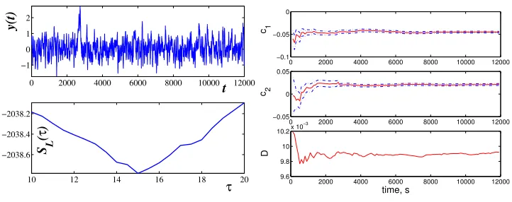
Fig. 1. Left column: the model signaly(t) (top), and inference of the time delayτ(bottom). Right column: inference of all the other parameters of the model (3.13). The original (exact) model parameters were:c1=−0.05,c2= 0.02,τ= 15,D= 0.01.

We evaluate this function for eachτ in a chosen range. Note thatSL(x|c) depends on τ via dependance on other inferred coefficients and first of all via dependance on noise intensityD. The global minimum of the log-likelihood function reveals the optimal value of the time delayτ. The corresponding to the optimal τ parameters

candDcan be picked up as a solution to the inference problem. Thus the outlined algorithm allows for a straightforward extension to encompass inference of stochastic models with unknown time delay.

We note that one of the advantages of the suggested algorithm is its high ef-ficiency. This makes it possible to achieve good convergence on very short time intervals (see for example parameter estimation of the Lorenz attractor in [10, 11]. Correspondingly, we can apply the algorithm to treat slowly varying parameters, as will be explained in more detail elsewhere. Nonetheless, the general problem of analysing non-stationary data with arbitrarily strong non-stationarity in all param-eters still remains an open challenge in nonlinear time-series analysis.

3. Inference of models with a time delay

In this section we verify numerically the algorithm outlined above. As an example we consider a simple model with a time delay

˙

y=c1z+c2yz+ξ(t), (3.13)

z=yτ =y(t−τ),

0 500 1000 1500 0.05

0.1 0.15

time, s

ventilation

0 0.05 0.1 0.15 0.2 0.25 0.3 0.35 0.4 0

0.02 0.04 0.06 0.08

frequency, Hz

PSD

Fig. 2. The ventilation signalV(t) (left) and its power spectral density (right).

τ = 15 is shown in Fig. 1(right). Again, one can see that the parameters converge to their correct values.

4. Inference of the Mackey-Glass model of the respiratory control system

Mackey and Glass proposed [6] a simple dynamical model of breathing control in which the human respiratory control was considered as a closed loop system with time delay. The model was subsequently extended [5] by Landa and Rosenblum to include the function of the brainstem respiratory center.

There are two state variables in the original Mackey-Glass model:V – ventila-tion, which is the volume of air that passes through the lungs during a single breath multiplied by the frequency of respiration; and x – the partial pressure of CO2 in the blood. The model was formulated as

˙

x=λ−αxV, (4.14)

V =Vm x n τ

Θn_−xn τ

, (4.15)

wherexτ =x(t−τ), andτ is the time delay.

This simple model is able to reproduce both normal and pathological Cheyne-Stokes breathing. The pathological or periodic breathing consists of short periods of deep and frequent breathing alternating with its complete cessation. One of the reasons for such behavior is abnormal blood circulation giving an increase in the time between oxygenation of blood in the lungs and stimulation of chemoreceptors in the brainstem. This corresponds to an increase of the time delayτ in the model (4.14)–(4.15).

1 1.5 2 2.5 3 3.5 4 -6450

-6350 -6250 -6150

τ, s

τ

)

S

( L

0 200 400 600 800 1000 1200 1400 1600 1800

0.03 0.035 0.04

c 1

0 200 400 600 800 1000 1200 1400 1600 1800

−0.9 −0.8 −0.7

c 2

0 200 400 600 800 1000 1200 1400 1600 1800

3 3.5 4

c 3

0 200 400 600 800 1000 1200 1400 1600 1800

0 0.000001 0.000002

time, s

D

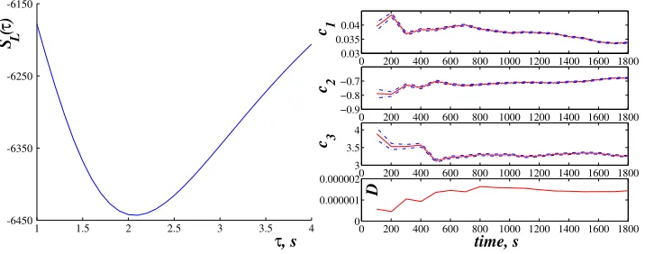
Fig. 3. Left: inference of the time delayτ for the modified Mackey-Glass model (4.18) from the constructed ventilation signalV(t). Right column: inference of the other model parameters from the constructed ventilation signalV(t) for the inferred time delay ofτ= 2.1 s.

we approximate the CO2response curve given in (4.15) as a linear function ofxτ

V(xτ) =a+bxτ. (4.16)

This simple approximation is justified if the control system is working close to the linear part ofV(xτ). The assumption is reasonable for normal and healthy breath-ing patterns, but it would be not correct for pathological Cheyne-Stokes breathbreath-ing, when the effect of saturation in the dependence of V(xτ) on xτ is significant. As-suming additive white Gaussian noise ξ(t), and substituting xτ from (4.16) into equation (4.14) we obtain a dynamical model for ventilation

˙

V =λb+αaVτ−αV Vτ+ξ(t), (4.17) whereVτ=V(t−τ) andτis the time delay. Finally, changing variables and notation we rewrite (4.17) as

˙

y=c1+c2z+c3yz+ξ(t), (4.18)

y=V, z=yτ=y(t−τ), hξ(t)i= 0, hξ(t)ξ(0)i=Dδ(t).

In order to apply the inference algorithm we require time series of the ventilation signal V(t). We construct it from noninvasively measured respiratory efforta _r(t) through the following procedure:

(i) We identify maxima and minima of ther(t) signal and construct their slowly varying envelopes. We suppose that the differenceR(t) between these two envelope functions is proportional to the volume of the air passing through the lungs during a single breath.

(ii) We construct the continuous respiration frequency functionF(t), interpo-lating the distances between successive points. The procedure is similar to

a

0 500 1000 1500 2000 0.06

0.08 0.1 0.12

time, s

y(t)

0 0.05 0.1 0.15 0.2 0.25 0.3 0.35 0.4 0

0.02 0.04 0.06 0.08

frequency, Hz

PSD

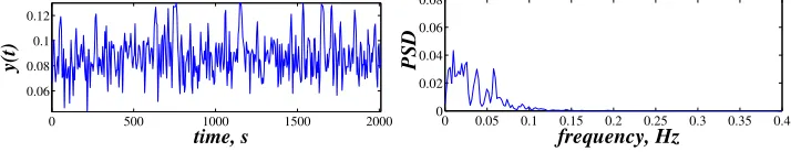
Fig. 4. Numerically generated ventilation signaly(t) from the model (4.18) based on the inferred parameters (left), and its power spectral density (right).

that used for construction of the heart rate variability (HRV) signal from the ECG.

(iii) Finally, the ventilation signalV(t) is computed as the product ofR(t) and

F(t). The signal and its power spectral density (PSD) are shown in Fig. 2. Following the procedure described previously we infer parameterscandD for a set of τ in a range from 0 s to 35 s. The behavior of the log-likelihood function near the minimum is shown in Fig. 3(left). The result of inference of the model (4.18) for the optimal (inferred) value of τ = 2.1 s is shown in Fig. 3(right). The estimated parameters are:c1 = 0.034;c2=−0.68;c3= 3.25;D= 1.4×10−6. In order to get some sense of whether the inference was successful, we numerically generate time series of the model (4.18) using these inferred parameters.b_{Time series of the model} state variabley and its PSD are shown in Fig. 4. This result can be compared with the original ventilation signal in Fig. 2. One can see that the model produces very similar behavior to the original ventilation signal V(t), in spite of the fact that the inferred time delay parameter differs from that imposed in the original model [6, 5]. The question, whether this is due to simplification of the model, or indeed the inferred parameter corresponds to the physiological delay in the respiratory system, we leave for future research.

5. Summary and conclusions

We have demonstrated a new Bayesian inference technique and shown that it can successfully be applied to stochastic nonlinear systems with delay. It enables us to extract model parameters from measured time series. We have tested the scheme on a simple one-dimensional model with delay, and applied it to the Mackey– Glass model of respiratory control. For both systems the scheme converged well and yielded parameter values that were either correct or, in the latter case,

plau-b

sible. It seems, therefore, that it offers a promising way of inferring physiologically relevant parameters from measured cardiovascular data.

Much remains to be done, however, before the technique can routinely be applied to the range of physiological systems that we would like to investigate. For example, the scheme needs to be extended to treat the non-white noise commonly found in physiology. In the medium/longer term, we hope to be able to infer parameters and interaction constants in the coupled-oscillator model [13] of the cardiovascular system, leading in turn to improved early diagnosis and better assessment of the efficacy treatment, based on simple noninvasive measurements.

Acknowledgements

The research was supported by the Engineering and Physical Sciences Research Council (UK), Leverhulme Trust (UK), NASA Intelligent Systems/Intelligent Data Understanding program (USA), Ministry of Education, Science and Sport (Slovenia) and INTAS.

References

1. C. L. Bremer and D. T. Kaplan, Markov chain Monte Carlo estimation of nonlinear dynamics from time series,Physica D 160(2001) 116–126.

2. J.-M. Fullana and M. Rossi,Identification methods for nonlinear stochastic sys-tems,Phys. Rev. E 65(2002) 031107.

3. R. Graham,Path integral formulation of general diffusion processes, Z. Phys. B 26(1977) 281–290.

4. J. P. M. Heald and J. Stark,Estimation of noise levels for models of chaotic dynamical systems,Phys. Rev. Lett.84(1999) 2366–2369.

5. P. Landa and M. Rosenblum,Modified Mackey-Glass model of respiration con-trol,Phys. Rev. E 52 (1995) R36–R39.

6. M. C. Mackey and L. Glass, Oscillations and chaos in physiological control systems,Science 197(1977) 287–288.

7. A. J. McKane, H. C. Luckock and A. J. Bray,Path integrals and non-Markov processes. I. General formalism, Phys. Rev. A41(1990) 644–656.

8. P. E. McSharry and L. A. Smith, Better nonlinear models from noisy data: Attractors with maximum likelihood, Phys. Rev. Lett.83(1999) 4285–4288. 9. R. Meyer and N. Christensen, Bayesian reconstruction of chaotic dynamical

systems,Phys. Rev. E 62(2000) 3535–3542.

10. V. N. Smelyanskiy and D. G. Luchinsky,Inference of stochastic nonlinear os-cillators with applications to physiological problems, in Z. Gingl, J. M. San-cho, L. Schimansky-Geier and J. Kertesz (eds.),Noise in Complex Systems and Stochastic Dynamics II, (Proc. SPIE), vol. 5471 (SPIE, Bellingham) (2004) pp. 344–354.

Fast Bayesian inference of stochastic nonlinear systems (available at: http://arxiv.org/abs/cond-mat/0409282), Phys. Rev. E submitted (2004). 12. V. N. Smelyanskiy, D. A. Timucin, D. G. Luchinsky, A. Stefanovska, A.

Ban-drivskyy and P. V. E. McClintock,Time-varying cardiovascular oscillations, in N. S. Namachchivaya and Y. K. Lin (eds.), IUTAM Symposium on Nonlinear Stochastic Dynamics (Kluwer, Amsterdam) (2003) pp. 455–464.

13. A. Stefanovska and M. Braˇciˇc, Physics of the human cardiovascular system,