Modelling and Forecasting LKR/USD Monthly Exchange Rates using Constant Elasticity of Variance (CEV) Model

Modelling and Forecasting LKR/USD Monthly Exchange

Rates using Constant Elasticity of Variance (CEV) Model

W.M.H.N. Weerasinghe

Department of Mathematics, University of Kelaniya

DOI: 10.29322/IJSRP.8.4.2018.p7620

http://dx.doi.org/10.29322/IJSRP.8.4.2018.p7620

Abstract- This paper model and forecast monthly exchange rates of US Dollar to Sri Lankan Rupee using Constant Elasticity of

Variance (CEV) Model. In this study, five models are formulated considering five elasticity factors 0, 1 2� , 1, 3 2� and 2. Monthly

exchange rates from January, 1995 to December, 2016 were obtained from the official website of Central Bank of Sri Lanka. Among this data, 254 observations were used to estimate the parameters and other 10 observations were used to test the validity of the models. To estimate the parameters, maximum likelihood estimation method is used and the exchange rates are generated using Euler- Maruyama method. The Monte Carlo technique is used for simulation and the accuracy of the forecasts is compared with Root Mean Squared Error (RMSE) and Mean Absolute Percentage Error (MAPE). The model which has the minimum RMSE and MAPE is chosen as the best model to predict the monthly exchange rate of LKR/USD.

Index Terms- Constant Elasticity of Variance Model, Maximum likelihood estimation, Monte Carlo technique, Euler- Maruyama method, Exchange rate

INTRODUCTION

Most countries use their own currencies as a medium of exchange, similar to the Rupee in Sri Lanka and the Dollar in the United States. Whenever a country with its own unique currency has to make payments to other countries which have different currencies, it has to exchange its currency with other currencies at a given rate of exchange. The rate at which one currency may be exchanged against another is called “the exchange rate”. The exchange rate is formally defined as the number of units of one currency that can be exchanged for a unit of another [3]. Exchange rate is very important in financial market, because it determines the level of imports and exports. Hence modeling and forecasting exchange rate is most important for the people who are doing international businesses to minimize the risk.

There are two pure approaches to forecast foreign exchange rates, fundamental and technical approach. The fundamental approach is

based on a wide range of data regarded as fundamental economic variables that determine exchange rates. The technical approach focuses on a smaller subset of the available data. In general, it is based on price information. The analysis is "technical" in the sense that it does not rely on a fundamental analysis of the underlying economic determinants of exchange rates or asset prices, but only on extrapolations of past price trends. Technical analysis looks for the repetition of specific price patterns. Generally, econometric models, time series models or a combination of both methods are used to forecast the exchange rate.

Stochastic differential equation (SDE) models can be used in many fields of science especially in finance. Black-Scholes model is the famous model among them. The constant elasticity of variance (CEV) model is a diffusion model with the instantaneous volatility specified to be a power function of the underlying spot price.

In this research, LKR/USD exchange rate is modeled using the CEV model and forecast the exchange rate using that model. Five

elasticity factors 0, 1 2� ,1, 3 2� and 2 were considered and the best model is selected from these five models. Monthly exchange rates

I. LITERATUREREVIEW

In literature, many studies were carried out to model and forecast the exchange rate. Booth and Glassman (1987), compared the

exchange rate forecasting models considering forecast accuracy and profitability. Tenti (1996), proposed the use of recurrent neural

networks to forecast foreign exchange rates. Nabni et al. (1996), described how modern machine learning techniques can be used in conjunction with statistical methods to forecast short term movements in exchange rates. Vinod and Samantha (1997), applied eight SDE models to exchange rate dynamics and evaluated the best model. They used three estimation methods, generalized method of moments (GMM), small sigma asymptotic estimating function (SSA-EF) and numerical conditional variance (NCV) method. Soofi and Cao (1999), performed out-of-sample predictions on daily Peseta–Dollar spot exchange rates using a simple nonlinear deterministic technique of local linear predictor. Gencay (1999), investigated the predictability of spot foreign exchange rate returns from past buy-sell signals of the simple technical trading rules by using the nearest neighbors and the feed forward network regressions.

Majhi, Panda and Sahoo (2009), developed two novel ANN models, functional link artificial neural network (FLANN) and cascaded functional link artificial neural network (CFLANN) involving nonlinear inputs and simple ANN structure with one or two neurons. Rime, Sarno and Sojli (2010) examined the linkages between exchange rate movements, order flow and expectations of macroeconomic variables. Jalil and Fleriden (2010) explained the exchange rate movements in the Pakistan foreign exchange market using the market micro structure approach. Simpson and Grossman (2010) used a relative purchasing power parity (PPP) model to construct a time-varying equilibrium exchange rates.

Abdorrahman et al. (2011), developed three decision making models to maximize profit of trades during a specific period and forecasted the direction of exchange rate over a specific period on the basis of values of indicators in previous time period. Pacelli (2012) analyzed and compared different mathematical models such as artificial neural networks, ARCH and GARCH models. Irena and Andrius (2013) discussed the advantages and drawbacks of the main fundamental exchange rate forecasting models. Yuan (2013), presented the polynomial smooth support vector machine (PSSVM) learning model. Minakhi et al. (2014), proposed a hybrid prediction model by combining an adaptive autoregressive moving average (ARMA) architecture and differential evolution (DE) based training of its feed-forward and feed-back parameters. Mehreen et al. (2014), explored Neuro- evolution and evaluated for its application in devising prediction models for foreign currency exchange rates. Tlegenova (2015), modeled yearly exchange rates between USD/KZT, EUR/KZT and SGD/KZT, and compared the actual data with developed forecasts using time series analysis over the period from 2006 to 2014. Urrutia et al. (2015), formulated a mathematical model to forecast exchange rate of the Philippines from the 1st Quarter of 2015 up to the 4th Quarter of 2020 using Autoregressive integrated Moving Average (ARIMA).

II. THE METHODOLOGY

The monthly exchange rate of LKR/USD for the period from January, 1995 to December, 2016 is represented in Figure 1. It can be observed that there is an upward trend of monthly exchange rate of LKR/USD in this period.

0.0000 20.0000 40.0000 60.0000 80.0000 100.0000 120.0000 140.0000 160.0000

1995 1995 1996 1997 1997 1998 1999 1999 2000 2001 2001 2002 2003 2003 2004 2005 2005 2006 2007 2007 2008 2009 2009 2010 2011 2011 2012 2013 2013 2014 2015 2015 2016

The diffusion process of 𝑋(𝑡) at time 𝑡 in a CEV model can be expressed as,

𝑑𝑋(𝑡) =𝜇𝑋(𝑡)𝑑𝑡+𝜎�𝑋(𝑡)�𝛽�2_{𝑑𝑊(𝑡) 0≤ 𝛽 < 2 (1)}

where 𝑋(𝑡) is the exchange rate at month 𝑡, 𝜇𝑋(𝑡) is the drift coefficient, 𝜎�𝑋(𝑡)�

𝛽 2 �

is the diffusion coefficient, 𝑊(𝑡) is a Weiner

process and 𝛽 is the elasticity factor. If 𝛽= 2, the CEV model returns to the conventional Black–Scholes model in which the variance

rate is independent of the stock price. If 𝛽= 0, it is the Ornstein–Uhlenbeck model.

The solution of the equation (3.1) can be approximated using Euler-Maruyama method and it is given by,

𝑋(𝑡) =𝑋(𝑡 −1) +𝜇𝑋(𝑡 −1)∆𝑡+𝜎𝑋(𝑡 −1)𝛽�2(𝑊(𝑡)− 𝑊(𝑡 −1)) (2)

In this research, five cases of 𝛽 were considered. They are 0,1

2, 1, 3

2 and 2. First of all, the parameters of the equation (1) must be

calculated. For this purpose, maximum likelihood estimation method [1] is used.

Let 𝑥₀,𝑥₁,𝑥₂, . . . ,𝑥_𝑁 are observed values of 𝑋(𝑡) at the respective uniformly distributed times 𝑡_𝑖 =𝑖𝛥𝑡 for 𝑖 = 0, 1, . . . ,𝑁 where,

𝛥𝑡 = 𝑇/𝑁. Let 𝑝(𝑡_𝑘,𝑥_𝑘|𝑡_𝑘−1,𝑥_𝑘−1; 𝜃) be the transition probability density of (𝑡_𝑘,𝑥_𝑘) starting from (𝑡_𝑘−1,𝑥_𝑘−1) given the vector𝜃.

Suppose that the density of the initial state is 𝑝₀(𝑥₀|𝜃).

In maximum likelihood estimation of 𝜃, the joint density

𝐷(𝜃) =𝑝0(𝑥0|𝜃)� 𝑝(𝑡𝑘,𝑥𝑘|𝑡𝑘−1,𝑥𝑘−1; 𝜃) 𝑁

𝑘=1

is maximized over 𝜃 ∈ ℝ𝑚 . It is more convenient to minimize the function

𝐿(𝜃) = −𝑙𝑛 (𝐷(𝜃)) which has the form

𝐿(𝜃) =−ln�𝑝0(𝑥0|𝜃)� − �ln�𝑝(𝑡𝑘,𝑥𝑘|𝑡𝑘−1,𝑥𝑘−1; 𝜃)� 𝑁

𝑘=1

One difficulty in finding the optimal value 𝜃∗ is that the transition densities are not generally known. However, by considering the

Euler approximation and letting 𝑋(𝑡_𝑘−1) = 𝑥_𝑘−1 at 𝑡=𝑡_𝑘−1

𝑋(𝑡𝑘) ≈ 𝑥𝑘−1 + 𝜇𝑥𝑘−1𝛥𝑡 + 𝜎𝑥𝑘−1 𝛽

2 �_{√𝛥𝑡𝜂}

𝑘

where 𝜂_𝑘~𝑁(0,𝛥𝑡).

This implies that

𝑝(𝑡𝑘,𝑥𝑘|𝑡𝑘−1,𝑥𝑘−1; 𝜃) = 1

�2𝜋𝜎𝑘2𝑒𝑥𝑝 �

−(𝑥𝑘− 𝜇𝑘)2

2𝜎𝑘2 �

where 𝜇_𝑘= 𝑥_𝑘−1 + 𝜇𝑥_𝑘−1𝛥𝑡 and 𝜎_𝑘 =𝜎𝑥_𝑘−1𝛽�2_√𝛥𝑡.

This transition density can be substituted into the expression for 𝐿(𝜃) which can subsequently be minimized over ℝ𝑚.

Then, the parameters 𝜇̂ and 𝜎� can be calculated using the equations:

𝜇̂=∑

(𝑥𝑘+1−𝑥𝑘)

𝑥𝑘𝛽−1

𝑁 𝑘=0

∆𝑡 ∑𝑁𝑘=0𝑥𝑘2−𝛽

and

𝜎�=�∑ 𝑥𝑘+1�𝑥𝑘−𝛽 2

� _{−(1 +𝜇∆𝑡)𝑥} 𝑘1−𝛽 2��

2 𝑁

𝑘=0

∆𝑡

After estimating parameters, sample paths for the exchange rates can be generated for each value of 𝛽. To simulate these sample paths, Monte Carlo method is used. Monte Carlo means using random numbers as a tool to compute something that is not random. It can be used to solve any problem having a probabilistic interpretation. By the law of large numbers, integrals described by the expected value of some random variable can be approximated by taking the empirical mean of independent samples of the variable.

As an example, let 𝑋 be a random variable and write its expected value as𝐴=𝐸(𝑋). If we can generate 𝑋₁,𝑋₂, … ,𝑋_𝑛 , 𝑛 independent

random variables with the same distribution, then we can make the approximation,

𝐴�𝑛=1_{𝑛 � 𝑋}𝑖 𝑛

𝑖=1

.

By law of large numbers, 𝐴� → 𝐴_𝑛 as𝑛 → ∞.𝑋_𝑖 and𝐴�_𝑛 are random and could be different each time we run the program. Still, the

target number 𝐴 is not random.

In this research work, forecasting is an important task. According to the five CEV models which are considered, future exchange rates can be forecasted using Monte Carlo simulation. Finally, the accuracy of forecasting is calculated using two methods, root mean square error (RMSE) and mean absolute percentage error (MAPE). The equations are given by,

𝑅𝑀𝑆𝐸=��(𝑥𝑖− 𝑥_𝑚�𝚤)2

𝑚

𝑖=1

and

𝑀𝐴𝑃𝐸=��∑ �

𝑥𝑖−𝑥�𝚤

𝑥𝑖 �

𝑚

𝑖=1 �

𝑚

� �× 100

where 𝑥_𝑖 is the observed value, 𝑥�_𝚤 is the forecasted value at time 𝑡=𝑖 and 𝑚 is the number of observations.Minimum value of these

values indicate the best model.

III. RESULTSANDFINDINGS

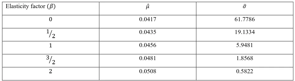
In this research, five CEV models are considered. According to the value of elasticity factor(𝛽), parameter estimations of each CEV

model is given in the Table I. To estimate the parameters, 254 observations are used.

Table I: Estimated Parameter Values for Five CEV Models

Elasticity factor (𝛽) 𝜇̂ 𝜎�

0 0.0417 61.7786

1 2

� 0.0435 19.1334

1 0.0456 5.9481

3 2

� 0.0481 1.8568

2 0.0508 0.5822

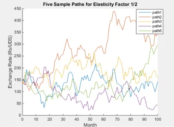
Figure 2: Five Sample Paths for the CEV Model 𝒅𝑿(𝒕) =𝟎.𝟎𝟒𝟏𝟕𝑿(𝒕)𝒅𝒕+𝟔𝟏.𝟕𝟕𝟖𝟔𝒅𝑾(𝒕)

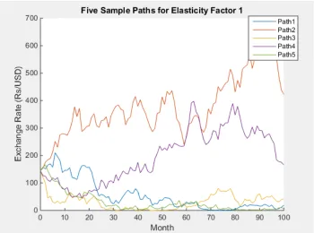
Figure 4: Five Sample Paths for the CEV Model 𝒅𝑿(𝒕) =𝟎.𝟎𝟒𝟓𝟔𝑿(𝒕)𝒅𝒕+𝟓.𝟗𝟒𝟖𝟏�𝑿(𝒕)�𝟏�𝟐𝒅𝑾(𝒕)

IV.

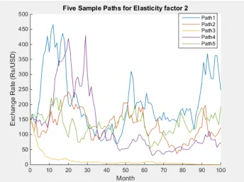
Figure 6: Five Sample Paths for the CEV Model 𝒅𝑿(𝒕) =𝟎.𝟎𝟓𝟎𝟖𝑿(𝒕)𝒅𝒕+𝟎.𝟓𝟖𝟐𝟐𝑿(𝒕)𝒅𝑾(𝒕)

In this study, LKR/USD monthly exchange rates for nine months are forecasted by considering the initial value as 143.9594 Rs/$ which is the exchange rate of March, 2016.

The generated monthly exchange rates of a time point is different to one sample path to another. Hence by generating one sample path, a fixed value for the exchange rate cannot be obtained. Because of that, Monte- Carlo simulation is used to obtain the convergent monthly exchange rate. Figure 7 to Figure 11 illustrate the convergence of exchange rate when the large number of sample paths are generated.

Figure 8: Convergence of Exchange Rate on April, 2016 for the model

𝒅𝑿(𝒕) =𝟎.𝟎𝟒𝟑𝟓𝑿(𝒕)𝒅𝒕+𝟏𝟗.𝟏𝟑𝟑𝟒�𝑿(𝒕)�𝟏�𝟒_{𝒅𝑾(𝒕)}

Figure 10: Convergence of Exchange Rate on April, 2016 for the model 𝒅𝑿(𝒕) =𝟎.𝟎𝟒𝟖𝟏𝑿(𝒕)𝒅𝒕+𝟏.𝟖𝟓𝟔𝟖�𝑿(𝒕)�𝟑�𝟒𝒅𝑾(𝒕)

By generating 200000 sample paths and taking the average of each point forecasted exchange rates are obtained. Table II represents the actual exchange rates and forecasted values for each model from April, 2016 to December, 2016.

Table II: Actual and Forecasted LKR/USD Exchange Rates from April, 2016 to December, 2016

Month Actual 𝜷=𝟎 𝜷=𝟏/𝟐 𝜷=𝟏 𝜷=𝟑/𝟐 𝜷=𝟐

03/2016 143.9594 143.9594 143.9594 143.9594 143.9594 143.9594

04/2016 143.9001 144.4051 144.5337 144.5532 144.4990 144.4974

05/2016 145.6502 144.8608 145.0134 145.0565 145.0581 145.0748

06/2016 145.2836 145.3562 145.5455 145.5918 145.6683 145.7518

07/2016 145.4070 145.8443 146.0579 146.1818 146.2689 146.3140

08/2016 145.6010 146.3502 146.5258 146.7334 146.8723 146.8614

09/2016 145.7849 146.8095 147.0654 147.2083 147.4450 147.3881

10/2016 146.8723 147.3390 147.6002 147.7664 148.0006 148.0006

11/2016 147.7710 147.9532 148.1652 148.2576 148.6318 148.6318

12/2016 148.8820 148.5570 148.7373 148.8140 149.1268 149.2442

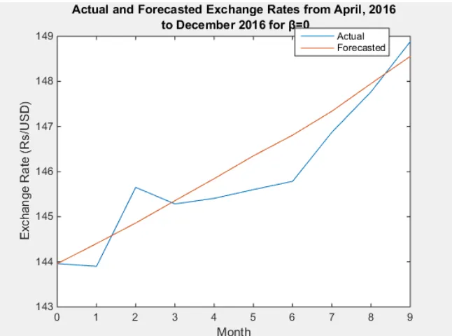
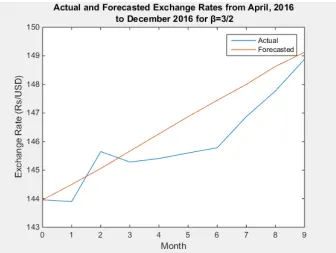
Graphically, The Actual and forecasted exchange rates for each model can be compared as follows:

Figure 13: Actual Rates and Forecasted Rates for the CEV Model

𝒅𝑿(𝒕) =𝟎.𝟎𝟒𝟑𝟓𝑿(𝒕)𝒅𝒕+𝟏𝟗.𝟏𝟑𝟑𝟒�𝑿(𝒕)�𝟏�𝟒_{𝒅𝑾(𝒕)}

Figure 15: Actual Rates and Forecasted Rates for the CEV Model 𝒅𝑿(𝒕) =𝟎.𝟎𝟒𝟖𝟏𝑿(𝒕)𝒅𝒕+𝟏.𝟖𝟓𝟔𝟖�𝑿(𝒕)�𝟑�𝟒𝒅𝑾(𝒕)

Among these five CEV models, the best model can be selected by checking forecasting accuracy measures RMSE and MAPE. Table III represented RMSE and MAPE values for each model.

Table III: RMSE and MAPE Values for Five CEV Models

𝜷 RMSE MAPE

0 0.5516 0.3113

1/2 0.6709 0.3862

1 0.7631 0.4321

3/2 0.8970 0.5173

2 0.8853 0.5210

According to the Table 3, the minimum RMSE and MAPE values can be observed when𝛽= 0. Therefore it can be concluded that the

best CEV model to forecast LKR/USD exchange rate among the five models is the model which has elasticity factor 0. Hence, the best CEV model is,

𝑑𝑋(𝑡) = 0.0417𝑋(𝑡)𝑑𝑡+ 61.7786𝑑𝑊(𝑡) It can be observed that the model is similar to the Ornstein- Uhlenbeck model.

IV. CONCLUSION

According to the results and findings, it can be concluded that the best model to predict LKR/USD monthly exchange rates from April, 2016 to December, 2016 is Ornstein-Uhlenbeck model. The best model may be changed to another model if one consider another data set. Because of that, by updating the exchange rates one can predict any future exchange rate using these models and the best model may be different to Ornstein-Uhlenbeck model.

In this research only five elasticity factors were considered. As a future research work, one can develop this study by considering more

than five elasticity factors. Since 𝛽 is continuous, if one can simulate results for more elasticity factors exchange rates can be predicted

more accurately.

REFERENCES [1] Allen E. (2007), “Modelling with Ito Stochastic Differential Equations”, Springer.

[2] Booth P., Glassman D. (1987), “Comparing Exchange Rate Forecasting Models: Accuracy versus Profitability”, International Journal of Forecasting, Vol. 3, Issue I, 65-79

[3] Central Bank of Sri Lanka (2006), “Exchange Rate”, Pamphlet Series, No. 03.

[4] Gencay R. (1999), “Linear, non-linear and essential foreign exchange rate prediction with simple technical trading rules”, in Journal of International Economics, Vol.47, 91–107.

[5] Haeri A., Rabbani M., Habibnia A. (2011), “The Proposed Mathematical Models for Decision-Making and Forecasting on Euro-Yen in Foreign Exchange Market”, Iranian Economic Review, Vol.16, No.30.

[6] Jalil A., Feridun M. (2010), “Explaining exchange rate movements: an application of the market microstructure approach on the Pakistani foreign exchange market”,

The Journal of Developing Areas, Vol. 44, Issue 1, 255-265.

[7] Lo C.F., Yuen P.H. (2000), “Constant Elasticity of Variance Option Pricing Model with Time-dependent Parameters”, International Journal of Theoretical and Applied

Finance Vol. 3, Issue 4 , 661–674.

[8] Macerinskiene I., Balciunas A. (2013), “Fundamental Exchange Rate Forecasting Models. Advantages and Drawbacks”, KSI Transactions on knowledge Society, Vol. 6, Issue 3, 9-17.

[10 ] Nabney I., Dunis C., Dallaway R., Leong S., Redshaw W. (1996), “Leading Edge Forecasting Techniques for Exchange Rate Prediction”, Forecasting Financial Markets. Exchange Rates and Asset Management, John Wiley & Sons, Chichester.

[11] Pacelli V. (2012), “Forecasting Exchange Rates: a Comparative Analysis”, International Journal of Business and Social Science Vol. 3 No. 10, 145-156.

[12] Rehman M., Khan G.M, Mahmud S.A. (2014), “Foreign Currency Exchange Rates Prediction Using CGP and Recurrent Neural Network”, IERI Procedia, Vol. 10, 239- 244

[13] Rime D., Sarno L., Sojli E. (2010), “Exchange rate forecasting, order flow and macroeconomic information”, Journal of International Economics, 72-88.

[14] Rout M., Majhi B., Majhi R., Panda G. (2014), “Forecasting of currency exchange rates using an adaptive ARMA model with differential evolution based training”,

Journal of King Saud University –Computer and Information Sciences, Vol 26, 7-18

[15] Simpson, M.W., Grossman, A. (2010). “Can a Relative Purchasing Power Parity-Based Model Outperform a Random Walk in Forecasting Short-Term Exchange \

Rates?:” International Journal of Finance and Economics, Vol. 16, Issue 4, 375-392.

[16] Singh V.K. and Ahmad N. (2011), “Forecasting Performance of Constant Elasticity of Variance Model: Empirical Evidence from India”, The International Journal

of Applied Economics and Finance, 5: 87-96.

[17] Soofi A. S., Cao L. (1999), “Nonlinear deterministic forecasting of daily peseta-dollar exchange rate”, in Economic Letters, Volume 62, pp.175–188. [18] Tenti P. (1996), “Forecasting foreign exchange rates using recurrent neural networks”, Applied Artificial Intelligence, Volume 10, pp. 567–581. [19] Tlegenova D. (2015), “Forecasting Exchange Rates Using Time Series Analysis: The sample of the currency of Kazakhstan”, Cornell University Library. [20] Urrutia J.D., Olfindo M.L.T., Tampis R. (2015), “Modelling and Forecasting the exchange Rate of the Philippines: A Time Series Analysis”, American Research Thoughts, Vol. 1, Issue 9.

[21] Vinod H.D. (1997), “Exchange Rate Dynamics Using GMM, Estimating Function and Numerical Conditional Variance Methods”, 17th Annual International Symposium on Forecasting, 1997.

[22] Yuan Y. (2013), “Forecasting the movement direction of exchange rate with polynomial smooth support vector machine”, Journal of Mathematical and Computer Modelling, Vol. 57 (3-4), 932-940.

AUTHORS

First Author – W.M.H.N. Weerasinghe, BSc (Hons.) in Mathematics, University of Kelaniya, [email protected] .