Coupling of a time domain boundary element method to compliant surface models

Coupling of a time domain boundary 

element method to compliant surface 

models

Hargreaves, JA and Cox, TJ

Title Coupling of a time domain boundary element method to compliant surface  models

Authors Hargreaves, JA and Cox, TJ

Type Conference or Workshop Item

URL This version is available at: http://usir.salford.ac.uk/id/eprint/19381/ Published Date 2010

USIR is a digital collection of the research output of the University of Salford. Where copyright  permits, full text material held in the repository is made freely available online and can be read,  downloaded and copied for non­commercial private study or research purposes. Please check the  manuscript for any further copyright restrictions.

Coupling of a time domain boundary element method to

compliant surface models

Jonathan A. HARGREAVES a and Trevor J. COX a

a

Acoustics Research Centre, University of Salford, Salford, M5 4WT, UK, e-mail: [email protected]

ABSTRACT

The Boundary Element Method (BEM) can be used to predict the scattering of sound in rooms. It reduces the problem of modelling the volume of air to one involving only the surfaces; hence the number of unknowns scales more favourably with problem size and frequency than it does for volumetric methods such as FEM and FDTD. The time domain BEM predicts the transient scattering of sound, and is usually solved in an iterative manner by marching on in time from known initial conditions.

Accurate representation of surface properties is crucial to obtain realistic simulations and the use of surface impedance is an established solution to this for frequency-domain problems. Recent research has successfully coupled digital filter representations of surface impedance to FDTD models, but the best way of achieving this for time domain BEM is currently

1. INTRODUCTION

The Boundary Element Method (BEM) has been shown to be an excellent choice for simulation in Room Acoustics when the priority is to predict scattering from a small object extremely accurately [1]. In the BEM only the boundaries between obstacles and air are modelled as it is known how sound travels unobstructed. This produces smaller, simpler meshes compared to volumetric methods, such as finite element method and Finite Difference Time Domain (FDTD), and permits an unbounded volume of air to be modelled, making it ideal for free-field scattering scenarios. Most BEMs assume harmonic excitation so the unknowns are time invariant and complex. Whilst this frequency domain analyses is a useful tool, the transient behaviour witnessed in the real world may only be recovered by solving many frequency domain models and then applying an inverse discrete Fourier transform. Accordingly applications such as auralisation have driven an interest in time domain modelling and many geometric, and more recently FDTD, algorithms have been published in pursuit of this. The time invariant assumption may also be dropped from the BEM formulation, leading to the time domain BEM as investigated herein. This approach was first published by Friedman and Shaw in 1962 [2], however computational cost and stability issues have plagued the method and commercial implementations have appeared only very recently [3]. Other work has focussed on extending the method to model features commonly found in room acoustics scenarios, for example the thin fins that occur on Schroeder Diffusers [4]. An accurate and efficient way to represent non-rigid obstacles, such as porous absorbent, is also crucial to obtaining realistic simulations. Surface impedance is typically used to characterise this behaviour in the frequency domain and is ideally suited to use with the frequency domain BEM; an equivalent time domain model is sought. Differential boundary conditions may be used to model simple compliant materials such as frequency-invariant absorption [5] [6] and limp membranes [7], but finding such models from arbitrary surface impedance data is more complicated [8]. Instead, various researchers tackling this challenge for FDTD have turned to digital filter representations [9] [10] [11], and this paper adapts the same approach to time domain BEM.

2. BOUNDARY INTEGRAL FORMULATION

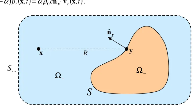
A BEM to model scattering from an object has three distinct phases: first the sound incident on the object is calculated, then the total sound at the surface of the object is solved for by considering the mutual interactions of parts of the surface S, and finally the scattered sound is calculated from this total surface sound. The scattered sound arising as a consequence of total sound on a surface is described by the Kirchhoff Integral Equation (KIE); this is the

foundation of the time domain BEM:

( )

=

_∫∫

[

( )

∗ ⋅∇

(

)

−

(

)

∗ ⋅∇

( )

]

S

t t

s x,t

ϕ

y,t nˆy yg R,t g R,t nˆy y

ϕ

y,t dy

ϕ

(1)

( )

t

( )

t

p x, ₌₋

ρ

₀

ϕ

& x, ₍₂₎

( )

x,t

( )

x,t

v =∇

ϕ

(3)

and 3, where ρ0 and c are the density of and speed of sound in air respectively. A dot above a quantity represents temporal differentiation and temporal convolution is represented by∗.

ϕ

_s

is the scattered sound and

ϕ

_t is the total sound. nˆ is the surface normal vector at _y y and g(R,t) is the time domain Greens function which describes how sound travels from a point source to an observer, which intuitively comprises a delay term as a numerator and a reduction in magnitude with distance as the denominator.

δ

( )

K _{is a dirac delta function:}

(

)

(

)

R c R t t R g

π

δ

4

, = − (4)

If x approaches S then the total surface sound may be solved for. However, rather than use this scheme directly it has been shown [12,13] that stability may be improved by using a variant called the Combined Field Integral Equation (CFIE), which is equivalent to the frequency domain Burton and Miller method [14] and will be used herein:

[image:4.595.128.462.304.486.2]

(

1−

α

) ( )

p_t x,t =

α

ρ

₀cnˆ_x⋅v_t

( )

x,t . (5)

Figure 1. A scattering problem comprising an obstacle in a connected medium.

3. SURFACE REFLECTANCE BOUNDARY CONDITION MODEL

In time harmonic models the concept of surface impedance convenient abstracts the behaviour of the material into a frequency dependent complex scalar, defined at the ratio of total

pressure to the inward component of total particle velocity:

( )

ω Pt

( )

ω Vtin

( )

ω

Z = , (6)

The same relationship may be stated in the time domain as pt

( )

t =vt,in

( ) ( )

t ∗z t . However, a

( )

t

z found by inverse discrete Fourier transform of Z

( )

ω

is typically non-compact in time and requires future values ofvt,in

( )

t . This is due to the aggregation of cause and effect in the quantities p_t and v_t,in, and makes it unsuitable for use with a time-marching solver. It has been suggested [15] that a convolution between waves travelling perpendicularly into and out of the body may be a more robust approach, and this concept has been developed for BEM for

−

Ω

x R y

y

nˆ

∞

S

+

Ω

the special case of obstacles with wells that are narrow with respect to wavelength [16]. This may be written in the time domain as:

( )

t in

( )

t w

( )

t

out =ϕ ∗

ϕ (7)

where the time invariant surface reflection kernel w

( )

t is typically compact in time and expresses ϕout using only past values of ϕin, hence is suitable for use with a time-marching

solver. The equivalent frequency domain statement involves the surface reflection kernel W:

( )

ω _in

( ) ( )

ωW ω

out =Φ

Φ (8)

In the special case of a well the surface reflection kernel could be analytically identified as a delayed delta function and readily incorporated into the integration kernels. However for an arbitrary material this is not the case so an alternate strategy is required. Explicit convolution (as Eq. 7) is computationally expensive, making recursive digital filters an attractive option. As will be seen in the next section this is particularly convenient since the Marching On in Time (MOT) solver already demands the histories of the surface quantities, and these can be used to implement the digital filters. The frequency domain surface reflection coefficient is used transformed into a z-domain filter definition and this in turn defines the difference equation for the boundary condition filter:

( )

( )

( )

( )

( )

( )

( )

( )

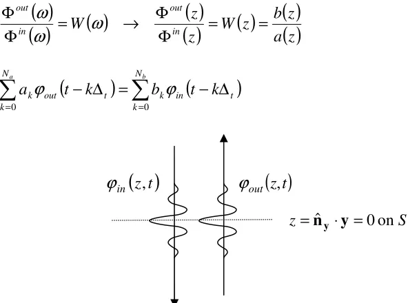
z a z b z W z z W _in out in out = = Φ Φ → = Φ Φ ω ω ω (9)

(

)

∑

(

)

∑

= = ∆ − = ∆ − b a N k t in k N k t out

k t k b t k

a

0 0

ϕ

[image:5.595.111.407.383.603.2]

ϕ

(10)

Figure 2. Plane waves propagating in and out of the obstacles perpendicular to S.

4. DISCRETISATION SCHEME AND SOLVER

In order to solve for the surface quantities numerically a discrete representation is required. The discretisation scheme herein uses as a weighted sum of basis functions where the boundary is partitioned into elements over which sound is considered constant within an instant and interpolated by a piecewise cubic polynomial in time. Spatial resolution is defined by element size and temporal resolution by the time-step duration ∆t.

( )

zt out , ϕ

( )

z t

in , ϕ

In the Marching On in Time (MOT) solver the discretisation weights are moved outside the integral of the KIE, creating a weighted sum of integrals that are dependent only on the surface geometry and independent of system excitation. Upon evaluation these integrals become interaction coefficients Zl that express scattered sound from the discretisation weights wj, creating a matrix equation that is solved from known initial conditions. Causality dictates that past surface sound cannot be changed and future sound is irrelevant, hence at each time-step tj = j∆t the algorithm is only solving for the current unknown weights. Because the surface model involves incoming and outgoing waves, each term appears twice (except the excitation vector ej):

∑

∑

= − = − − − = + l l N l out l j out l N l in l j in l j out j out in j in 1 1 0

0w Z w e Z w Z w

Z (11)

This matrix equation has twice as many unknowns as knowns so cannot be solved on its own, so the surface reflectance relationship must also be utilized. Observation that the outgoing wave must be a causal function of the incoming wave prompts rearrangement of Eq. 10 to evaluate wout_j :

∑

∑

= − = − − = k k N k out k j k N k in k j k out j 1 0

0w B w A w

A where

    = = otherwise 0 if ; , ; n m a_kn

n m k

A (12)

Under normal circumstances the filters are expected to be normalised to A0 = I. Together

these yield a solvable system of matrix equations.

5. SIMULATIONS AND RESULTS

Details and results of the simulations will be included in the lecture presentation. These will focus on verification on flat homogenous obstacles, as is typical for the equivalent published FDTD models, including porous absorbers. In addition the algorithm with also be verified against a frequency domain BEM model.

4. CONCLUSIONS

This paper has outlined a scheme for integrating a recursive digital filter model of the reflectance of a surface into a time domain BEM algorithm.

5. REFERENCES

[1] T. J. Cox and Y. W. Lam: “Prediction and Evaluation of the Scattering from Quadratic Residue Diffusers”, J. Acoust. Soc. Am. Vol. 95 (1), 1994, pp. 297-305

[2] M. B. Friedman and R. P. Shaw, “Diffraction of Pulses by Cylindrical Obstacles of Arbitrary Cross Section”, J. Appl. Mech. Vol. 29, 1962, pp. 40 – 46

[4] J. A. Hargreaves and T. J. Cox: “A Transient Boundary Element Method for Acoustic Scattering from Mixed Regular and Thin Rigid Bodies”, Acta Acustica united with Acustica, Vol. 95, 2009, pp. 678 – 689

[5] T. Ha-Duong, B. Ludwig and I.Terrasse, “A Galerkin BEM for transient acoustic scattering by an absorbing obstacle”, Int. J. Numer. Meth. Engng. Vol. 57, 2003, pp. 1845 – 1882

[6] P. H. L. Gronenboom, “The applications of boundary elements to steady and unsteady potential fluid flow problems in two and three dimensions”, Appl. Math. Modelling Vol. 6, 1982. pp. 35 – 40

[7] R. P. Shaw, “Diffraction of Acoustic Pulses by Obstacles of Arbitrary Shape with a Robin Boundary Condition”, J. Acoust. Soc. Am. Vol. 41 (4A), 1967, 855 – 859

[8] C. K. W. Tam and L. Auriault, “Time-Domain Impedance Boundary Conditions for Computational Aeroacoustics”, AIAA J. Vol. 34 (5) 1996, 917 – 923

[9] K. Kowalczyk and M. Van Walstijn, “Modelling Frequency-Dependent Boundaries as Digital Impedance Filters in FDTD and K-DWM Room Acoustics Simulations” J. AES, Vol. 56 (7/8), 2008, pp. 569 – 583

[10] I. A. Drumm and Y. W. Lam: “Development and assessment of a finite difference time domain room acoustic prediction model that uses hall data in popular formats”, Proceedings, Internoise-Turkey, (2007)

[11] J. Escolano, J. J. López and B. Pueo, “Locally Reacting Impedance in a Digital Waveguide Mesh by Mixed Modeling Strategies for Room Acoustic Simulation”, Acta Acustica united with Acustica, Vol. 95 (6), 2009, pp. 1048 – 1059

[12] A. A. Ergin, B. Shanker and E. Michielssen, “Analysis of transient wave scattering from rigid bodies using a Burton-Miller approach”, J. Acoust. Soc. Am. Vol. 106 (5), 1999, pp. 2396 – 2404

[13] D. J. Chappell, P. J. Harris, D. Henwood and R. Chakrabarti, “A stable boundary integral equation method for modelling transient acoustic radiation”, J. Acoust. Soc. Am. Vol. 120 (1), 2006, 74 – 80

[14] A. J. Burton and G. F. Miller, “The application of integral equation methods to the numerical solution of some exterior boundary-value problems”, P. Roy. Soc. Lond. A. Mat. Vol. 323, 1971, pp. 201 – 210

[15] K.-Y. Fung, H. Ju, B.-P. Tallapragada, “Impedance and Its Time-Domain Extensions”, AIAA J. Vol. 38 (1), 2000, pp. 30 – 38