International Journal of Emerging Technology and Advanced Engineering
Website: www.ijetae.com (ISSN 2250-2459, UGC Approved List of Recommended Journal, Volume 8, Issue 4, April 2018)233
A Novel Approach to Detect Salient Region Automatically in an
Image via High-Dimensional Color Transform and Local
Spatial Support
Devireddy Prathyusha
1, S. Harshavardhan
21PG Scholar, 2 Asst. Professor, Department of ECE, Vignan’s Nirula Institute of Technology, Guntur, AP, India
Abstract— In this paper, it has been introduced that, a
novel approach to automatically detect salient regions in an image. The approach consists of global and local features, to compute a saliency map. Image matting refers to the problem of accurately extracting the foreground object from an image. It has been using a depth to assist color for improving the foreground object and generate trimap based color distribution of local unknown regions to make it cover foreground boundary. The first key idea of our work is to create a saliency map of an image by using a linear combination of colors in a high-dimensional color space Jiwhan Kim et al. [25]. The second key idea is to detect the foreground image by using the local spatial support. Finally it has been combined both the results to form final saliency map.
Keywords— Salient region detection, super-pixel, tri-map,
random forest, color channels, high-dimensional color space.
I. INTRODUCTION
Salient region detection is important in image understanding and analysis. Its goal is to detect salient regions in an image in terms of a saliency map, where the detected regions would draw humans’ attention. Salient region detection is used in many applications like photo rearrangement, segmentation, image retargeting, image thumb nailing, object recognition, video compression and image quality assessment.
[image:1.612.330.556.242.302.2]In this paper, it was proposed a novel approach to detect salient regions automatically in an image. Here it has been first estimates the approximate locations of salient regions by using a trimap. The tree-based classifier classifies each super-pixel as foreground, background or unknown this form a trimap. Here it was proposed two different techniques to estimate saliency map, high-dimensional color transform (HDCT)-based method and local spatial support method with little modifications from that of Jiwhan Kim et al. [25]. Here it was combined these two methods to get final saliency map.
Fig 1. Overview of our algorithm: (a) input image (b) Over segmentation to superpixels (c) Initial saliency trimap (d) Global salient region detection via HDCT (e) Local Salient region detection
via random forest (f) Our final saliency map.
Image matting targets to extract foreground object from an image accurately. The process of matting is mathematically modelled by considering the observed color Ip of a pixel p as a combination of foreground Fp and background Bp colors along with its alpha value αp.
(1
)
,
[0,1]
(1)
p p p p p p
I
F
B
This math model can be solved by adding constraint using trimap that consist of a mixture of foreground and background colors. Due to introducing trimap, Fp and Bp of an unknown pixel p can be estimated by samples of known foreground and known background. Then the αp of unknown pixel p can be calculated by eq(1)
The HDCT is a global method. The saliency map of HDCT is shown in fig 1(d). The local spatial support is a local method. In local method we use K nearest foreground/background superpixel as shown in fig 1(e). We combine the saliency maps from the HDCT method and the local spatial support method by weighted combination (Fig. 1 (f)).
II. INITIAL SALIENCY TRI-MAP GENERATION
International Journal of Emerging Technology and Advanced Engineering
Website: www.ijetae.com (ISSN 2250-2459, UGC Approved List of Recommended Journal, Volume 8, Issue 4, April 2018)234
(A)Super pixel Saliency Features:
As demonstrated in recent studies [17] - [20], features from super pixels are effective and efficient for salient object detection. For an input image I, we first perform over-segmentation to form super pixels X = {X1… XN}. We use the SLIC super pixel [1] because of its low computational cost and high performance, and we set the number of super pixels to N = 500.
The location feature is used to focus more on objects that we used in foreground. Then, we concatenate the color features, as this is one of the most important cues in the human visual system and certain colors tend to draw more attention than others [19].
Next, we concatenate HOG features as this is one of the most effective measurements for the saliency feature, as demonstrated in [17]. In HOG feature we calculate the histogram value. The histogram features of the ith super
pixel is measured using the chi-square distance
between other super pixels’ histograms. It is defined as
2
1 1
(
)
(2)
(
)
i
N b
ik jk
H
j k ik jk
h
h
D
h
h
Where b is the number of histogram bins. In this work, it has been used eight bins for each histogram.
[image:2.612.332.556.481.579.2]For texture and shape features, we utilize the super pixel area, histogram of gradients (HOG), and singular value feature. The singular value feature (SVF) [10] is used to detect the blurred region from a test image because a blurred region often tends to be a background.
Table I
Comparision Of Trimap Performance On Msra-B Dataset [49]
Method Regression-based Classification-based
Foreground
precision 0.789 0.875
Background
precision 0.980 0.983
Error rate 0.032 0.019
Unknown rate 0.423 0.308
(B) Initial Saliency Trimap via Random Forest Classification:
Generally, the goal of trimap generation is to mark out the foreground boundary in which the alpha values are to be calculated. Therefore, we firstly use depth information to find out the target foreground. We use mean shift cluster method to segment the depth map into several blobs.
We take the blob with nearest depth and largest size as the target foreground of image matting. After that, we use the foreground depth as a threshold and generate a mask in which the foreground is labelled as 1 while the others are labelled as 0. Since the depth map contains noise and missing data, the found foreground is fairly rough. Therefore, we erode the mask to remove noise and dilate it several times to make true foreground regions are covered as much as possible in non-zero regions. The region got from dilation is the unknown region and labelled as 0.5. Thus, we get the initial trimap and can use it to calculate alpha matte for the image.
Table I shows a comparison of the trimap performance, in which the Fg. Precision (FP), Bg. Precision (BP), error rate (ER) are defined as below:
| { } { }|
(3) | { }|
C GT
p
C
F F
F
F
| { } { }|
(4) | { }|
C GT
p
C
B B
B
B
| ({
}
{
})
({
}
{
}) |
(5)
| { } |
C GT C GT
R
F
B
B
F
E
I
In which |·| denotes the number of pixels, FC and BC denote the foreground/background candidates, FGT and BGT
denote the ground-truth annotations’
foreground/background, respectively, and I denotes the whole image.
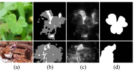
Fig 2. Some results of the initial saliency trimap. (a) Input Image (b) Binary Map without unknown region (c) our initial saliency trimap
with unknown region indicated in gray color. (d) Ground truth.
III. SALIENCY ESTIMATION FROM TRIMAP
International Journal of Emerging Technology and Advanced Engineering
Website: www.ijetae.com (ISSN 2250-2459, UGC Approved List of Recommended Journal, Volume 8, Issue 4, April 2018)235
(A) Global Saliency Estimation via HDCT
Colors are important cues in the human visual system. It is inconvenient to process colors in the RGB space as illumination and colors are nested here. Therefore, many different color spaces have been introduced, including YUV, YIQ, CIELab, and HSV.
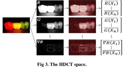
[image:3.612.65.270.279.392.2]As shown in Fig. 3. It is been concatenated only the nonlinear RGB transformed color space, because the effects of the coefficients of a linear transformed color space such as YUV/YIQ will be cancelled when we linearly combine the color coefficient to form our saliency map.
Fig 3. The HDCT space.
The concatenate different nonlinear RGB transformed color space representations to form a high-dimensional feature vector to represent the color of pixel.
To further enrich the representative power of our HDCT space, it has been applied power-law transformations to each color coefficient after normalizing the coefficient between [0, 1]. It is used three gamma values: {0.5, 1.0, and 2.0}.1 this resulted in a high-dimensional matrix to represent the colors of an image:
1 2 3 1
1 1 1 1
1 2 3 1
2 2 2 2
1 2 3 1
(6)
N l
N N N N
R
R
R
G
R
R
R
G
K
R
R
R
R
G
Here Ri and Gi denote the test image’s ith super pixel’s
mean pixel value of the R and G color channel,
respectively. By using 11 color channels such as RGB, CIELab, hue, and saturation, we can obtain an HDCT matrix K with l = 11 × 3 = 33.
To obtain saliency map, it has been utilized the foreground/background candidate color samples in our trimap to estimate an optimal linear combination of color coefficients to separate the salient region color and background color. It was formulated this problem as a l2 regularized least squares problem that minimizes
2 2 2 2
min || (
U K
||
|| ||
(7)
Where α ∈ Rl is the coefficient vector that one want to estimate, λ is a weighting parameter to control the magnitude of α, and is an M × l matrix with each row
of corresponding to color samples in the
foreground/background candidate regions:
1 2 3 1
1 1 1 1
1 2 3 1
1 2 2 1
1 1 1 1
1 2 3 1
(8)
FS FS FS FS
FSf FSf FSf FSf
BS BS BS BS
BSb BSb BSb BSb
R R R G
R R R G
K
R R R R
R R R G
Where, FSi and BSj denote the ith
foreground/background candidate super pixel among entire super pixels that are classified at the trimap generation step, respectively. M is the number of color samples in the
foreground/background candidate regions and f
and b denote the number of foreground/background regions, respectively, such that M = f + b. Jiwhan Kim et al. [25] stated that the following algorithm achieves the final saliency map.
Algorithm 1) HDCT-Based Saliency Estimation
Input: Initial trimap T and K
1) M ← f + b
2) Construct
K
R
M l3) Construct
1
M
U
R
4) Calculate
1
*
(
K K
TI
)
K U
T
5) Calculate 1
( ) *
l
G i i j j j
S X K
Output: saliency map SG
U is an M dimensional vector with value equal to 1 and 0 if a color sample belongs to the foreground/background candidate, respectively:
11 1
10 0
0
T M(9)
U
R
International Journal of Emerging Technology and Advanced Engineering
Website: www.ijetae.com (ISSN 2250-2459, UGC Approved List of Recommended Journal, Volume 8, Issue 4, April 2018)236
1
( )
* ,
1, 2,
(10)
l
G i i j j
j
S X
K
i
N
Fig 4. An illustration of local saliency features, Black, White and Gray regions denote background superpixels, foreground super pixels, and unknown superpixels, respectively. It has been useed K-nearest foreground superpixels and K-nearest background superpixels to calculate a feature vector.
(B) Local Saliency Estimation via Regression
The HDCT based method is easily effect of noise and texture so to overcome this limitation we present local spatial support. In this it was found K-nearest foreground and background superpixel as shown in fig 4.For each
super pixel Xi, we find the K-nearest
foreground/background super pixels are XFS =
{XFS1,XFS2...XFSK} ; XBS = {XBS1, XBS2...XBSK} respectively and we use the Euclidean distance between a super pixel Xi and super pixels XFS or XBS as features. The Euclidean distance to the K-nearest foreground/background is denoted as (dFSi∈ RK×1) and (dBSi∈ RK×1)
1 2
2 2
2 2
2 2
|| ||
|| ||
|| K||
i FSi
i FSi FSi
i FSi
p p
p p
d
p p
1
2
2 2
2 2
2 2
|| ||
|| ||
(11)
|| K||
i BSi
i BSi BSi
i BSi
p p
p p
d
p p
In which and denotes the jth nearest
[image:4.612.60.277.127.287.2]foreground/background super pixel from the ith super pixel.
Table II
Local Saliency Features That Are Used To Compute The Feature Vector For Each Superpixel
Feature Descriptions dim
Geodesic Distance Features Euclidean distance to K-nearest foreground superpixel
K
Euclidean distance to K-nearest background superpixel
K
Color Distance Features
color distance to K-nearest foreground
superpixel
8K
color distance to K-nearest background superpixel
8K
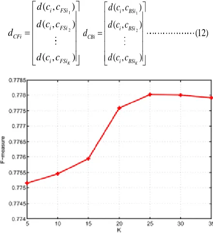
The feature vector of color distances from the ith super pixel to the K-nearest foreground (dCFi∈ R
8K×1 ) and background (dCBi∈ R8K×1) super pixels is defined as follows:
1
2
( ,
)
( ,
)
( ,
)
K
i FSi i FSi CFi
i FSi
d c c
d c c
d
d c c
1
2 ( , )
( , )
(12)
( , )
K
i BSi i BSi CBi
i BSi
d c c
d c c d
d c c
[image:4.612.332.552.356.596.2] [image:4.612.58.284.518.602.2]International Journal of Emerging Technology and Advanced Engineering
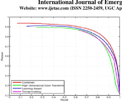
Website: www.ijetae.com (ISSN 2250-2459, UGC Approved List of Recommended Journal, Volume 8, Issue 4, April 2018) [image:5.612.64.278.108.287.2]237 Fig 6. Comparison of precision-recall curves of each step on the
MSRA-B dataset.
(C) Final Saliency Map Generation & Experimental Results:
After generating the global and the local saliency maps, they have been combined to generate the final saliency map. Therefore, combining the two maps is a significant step in our algorithm. Borji et al. [24] proposed two approaches to combine the two saliency maps. The first approach is to perform the pixel-wise multiplication of the two maps, as shown below:
1
( (
)
(
))
(13)
mult G L
S
p S
p S
Z
In which Z is a normalization factor, p(.) is a pixel-wise combination function, SG and SL is the global and local saliency result respectively.
The second approach is to combine the two maps using a summation:
1
( (
)
(
))
(14)
sum G L
S
p S
p S
Z
Based on Eq. (14), we adopt p(x) = exp(x)as a combination function to give greater weightage to the highly salient regions.
Finally, we defined the equation of the final saliency map combination as
1 2 3 4
1
(
(
)
(
))
(15)
final G L
S
w p w S
w p w S
Z
IV. EXPERIMENTAL RESULTS
(A). Performance Evaluation
In this study, it has been used two standard criteria for evaluating our salient region detection algorithm: precision-recall rate and F-measure rate.
1) Precision-Recall Evaluation:The precision is also called the positive predictive value, and it is defined as the ratio of the number of ground-truth pixels retrieved as a salient region to the total number of pixels retrieved as the salient region. The recall rate is also called the sensitivity, and it is defined as the ratio of the number of salient regions retrieved to the total number of ground-truth regions.
2) F-Measure Rate Evaluation: The second evaluation index is the F-measure rate. The F-measure combines the precision and the recall rate for a comprehensive evaluation. In this study, Jiwhan Kim et al. [25] it has been used the Fβ measure, as defined below:
2
2
(1 ) Pr
(16) Re
ecision Recall F
Precision call
As in previous methods [5], [6], [19], we used β2= 0.3.
(B) Result:
(C). Failure Cases
International Journal of Emerging Technology and Advanced Engineering
Website: www.ijetae.com (ISSN 2250-2459, UGC Approved List of Recommended Journal, Volume 8, Issue 4, April 2018) [image:6.612.58.281.130.248.2]238 Fig. 7. Some examples of failure cases. (a) Input images. (b) Our
initial trimap. (c) Our results. (d) Ground truth.
V. CONCLUSION
In this paper it has been clearly demonstrated a novel salient region detection method that estimates the foreground regions from a tri-map using two different methods: global saliency estimation via HDCT and local saliency estimation via regression. The tri-map based robust estimation overcomes the limitations of inaccurate initial saliency classification. As a result, this method achieves good performance and is computationally efficient in comparison to the state-of-the art methods Jiwhan Kim et al. [25]. In the future, it is possible for further modifications and updating by utilizing motion information and object detection result to improve the technology.
Acknowledgements
We are very much thankful to Mr.Jiwhan Kim, Mr. Dongyoon Han, Mr. Yu-Wing Tai, Mr. Junmo Kim[25] for their base paper which we used to do this project and the entire credit goes to them only.
REFERENCES
[1] R. Achanta, A. Shaji, K. Smith, A. Lucchi, P. Fua, and S. Süsstrunk, “SLIC superpixels compared to state-of-the-art superpixel methods,” IEEE Trans. Pattern Anal. Mach. Intell., vol. 34, no. 11, pp. 2274–2282, Nov. 2012.
[2] J. Kim, D. Han, Y.-W. Tai, and J. Kim, “Salient region detection via high-dimensional color transform,” in Proc. IEEE Conf. Comput. Vis. Pattern Recognit. (CVPR), Jun. 2014, pp. 883–890.
[3] A. Borji, M.-M. Cheng, H. Jiang, and J. Li. (2014). “Salient object detection: A survey.” [Online]. Available: http://arxiv.org/abs/1411.5878 [4] A. Borji, M.-M. Cheng, H. Jiang, and J. Li. (2015). “Salient object
detection: A benchmark.” [Online]. Available:
http://arxiv.org/abs/1501.02741
[5] R. Achanta, S. Hemami, F. Estrada, and S. Susstrunk, “Frequency-tuned salient region detection,” in Proc. IEEE Conf. Comput. Vis. Pattern Recognit. (CVPR), Jun. 2009, pp. 1597–1604.
[6] Q. Yan, L. Xu, J. Shi, and J. Jia, “Hierarchical saliency detection,” in Proc. IEEE Conf. Comput. Vis. Pattern Recognit. (CVPR), Jun. 2013, pp. 1155–1162.
[7] M.-M. Cheng, G.-X. Zhang, N. J. Mitra, X. Huang, and S.-M. Hu, “Global contrast based salient region detection,” in Proc. IEEE Conf. Comput. Vis. Pattern Recognit. (CVPR), Jun. 2011, pp. 409–416. [8] Z. Liu, R. Shi, L. Shen, Y. Xue, K. N. Ngan, and Z. Zhang,
“Unsupervised salient object segmentation based on kernel density estimation and two-phase graph cut,” IEEE Trans. Multimedia, vol. 14, no. 4, pp. 1275–1289, Aug. 2012.
[9] V. Navalpakkam and L. Itti, “An integrated model of top-down and bottom-up attention for optimizing detection speed,” in Proc. IEEE Conf. Comput. Vis. Pattern Recognit. (CVPR), Jun. 2006, pp. 2049–2056. [10] B. Su, S. Lu, and C. L. Tan, “Blurred image region detection and
classification,” in Proc. ACM Int. Conf. Multimedia, 2011, pp. 1397– 1400.
[11] R. O. Duda and P. E. Hart, Pattern Classification and Scene Analysis. New York, NY, USA: Wiley, 1973.
[12] Y.-S. Wang, C.-L. Tai, O. Sorkine, and T.-Y. Lee, “Optimized scale-andstretch for image resizing,” ACM Trans. Graph., vol. 27, no. 5, p. 118, Dec. 2008.
[13] J. Park, J.-Y. Lee, Y.-W. Tai, and I. S. Kweon, “Modeling photo composition and its application to photo re-arrangement,” in Proc. IEEE Int. Conf. Image Process. (ICIP), Sep./Oct. 2012, pp. 2741–2744. [14] A. Ninassi, O. Le Meur, P. Le Callet, and D. Barbba, “Does where you
gaze on an image affect your perception of quality? Applying visual attention to image quality metric,” in Proc. IEEE Int. Conf. Image Process. (ICIP), vol. 2. Sep./Oct. 2007, pp. II-169–II-172.
[15] L. Marchesotti, C. Cifarelli, and G. Csurka, “A framework for visual saliency detection with applications to image thumbnailing,” in Proc. IEEE Int. Conf. Comput. Vis. (ICCV), Sep./Oct. 2009, pp. 2232–2239. [16] L. Itti, “Automatic foveation for video compression using a
neurobiological model of visual attention,” IEEE Trans. Image Process., vol. 13, no. 10, pp. 1304–1318, Oct. 2004.
[17] H. Jiang, J. Wang, Z. Yuan, Y. Wu, N. Zheng, and S. Li, “Salient object detection: A discriminative regional feature integration approach,” in Proc. IEEE Conf. Comput. Vis. Pattern Recognit. (CVPR), Jun. 2013, pp. 2083–2090.
[18] F. Perazzi, P. Krahenbuhl, Y. Pritch, and A. Hornung, “Saliency filters: Contrast based filtering for salient region detection,” in Proc. IEEE Conf. Comput. Vis. Pattern Recognit. (CVPR), Jun. 2012, pp. 733–740. [19] X. Shen and Y. Wu, “A unified approach to salient object detection via
low rank matrix recovery,” in Proc. IEEE Conf. Comput. Vis. Pattern Recognit. (CVPR), Jun. 2012, pp. 853–860.
[20] C. Yang, L. Zhang, H. Lu, X. Ruan, and M.-H. Yang, “Saliency detection via graph-based manifold ranking,” in Proc. IEEE Conf. Comput. Vis. Pattern Recognit. (CVPR), Jun. 2013, pp. 3166–3173.
[21] A. Levin, A. Rav Acha, and D. Lischinski, “Spectral matting,” IEEE Trans. Pattern Anal. Mach. Intell., vol. 30, no. 10, pp. 1699–1712, Oct. 2008.
[22] T. Liu, J. Sun, N.-N. Zheng, X. Tang, and H.-Y. Shum, “Learning to detect a salient object,” in Proc. IEEE Conf. Comput. Vis. Pattern Recognit. (CVPR), Jun. 2007, pp. 1–8.
[23] L. Breiman, “Random forests,” Mach. Learn., vol. 45, no. 1, pp. 5–32, Oct. 2001.
[24] A. Borji, D. N. Sihite, and L. Itti, “Salient object detection: A benchmark,” in Proc. IEEE Eur. Conf. Comput. Vis. (ECCV), Oct. 2012, pp. 414–429.
![Table I Comparision Of Trimap Performance On Msra-B Dataset [49]](https://thumb-us.123doks.com/thumbv2/123dok_us/8679470.874304/2.612.332.556.481.579/table-i-comparision-trimap-performance-msra-b-dataset.webp)