ISSN: 1992-8645 www.jatit.org E-ISSN: 1817-3195
RECOGNIZING THE 2D FACE USING EIGEN FACES BY
PCA
M. JASMINE PEMEENA PRIYADARSINI1, K.MURUGESAN2, SRINIVASA RAO INABATHINI3, G.K RAJINI4, DINESH 5, AJAY KUMAR. R6
1356
School of Electronics Engineering, VIT University, Vellore, India
4
School of Electrical Engineering, VIT University, Vellore, India 2
Vel Tech High Tech Engineering College, Chennai, India.
ABSTRACT
Face Recognition is the process of identification of a person by their facial image. This technique makes it possible to use the facial images of a person to authenticate him into a secure system, for criminal identification, for passport verification etc. Face recognition approaches for still images can be broadly categorized into holistic methods and feature based methods . Holistic methods use the entire raw face image as an input, whereas feature based methods extract local facial features and use their geometric and appearance properties. The present thesis primarily focuses on Principal Component Analysis (PCA), for the analysis and the implementation is done in software, MATLAB. This face recognition system recognizes the faces where the pictures are taken by web-cam or a digital camera are given as test database and these face images are then checked with training image dataset based on descriptive features]. Descriptive features are used to characterize images. It describes how to build a simple, yet a complete face recognition ] system using Principal Component Analysis, a Holistic approach. This method applies linear projection to the original image space to achieve dimensionality reduction. The system functions by projecting face images onto a feature space that spans the significant variations among known face images. The significant features known as eigenfaces do not necessarily correspond to features such as ears, eyes and noses. It provides for the ability to learn and later recognize new faces in an unsupervised manner. This method is found to be fast, relatively simple, and works well in a constrained environment.
Keywords:-PCA, Eigen Faces, Eigenvalue, Eigenvector Face Space
1. INTRODUCTION
Face recognition systems have been grabbing high attention from commercial market point of view as well as pattern recognition field. Face recognition has received substantial attention from researches in biometrics, pattern recognition field and computer vision communities [1]. The face recognition systems can extract the features of face and compare this with the existing database [1] [6]. Face recognition has become an important issue in many applications such as security systems, credit card verification and criminal identification. For example, the ability to model a particular face and distinguish it from a large number of stored face models would make it possible to vastly improve criminal identification. Even the ability to merely detect faces, as opposed to recognizing them, can be important. Detecting faces in photographs for automating color film development can be very useful, since the effect of many enhancement and noise reduction techniques depends on the image content. Although [6] it is clear that people are
good at face recognition, it is not at all obvious how faces are encoded or decoded by the human brain. Human face recognition has been studied for more than twenty years. Unfortunately developing a computational model of face recognition is quite [6] difficult, because faces are complex, multi-dimensional visual stimuli. Therefore, face recognition is a very high level computer vision task, in which many early vision techniques can be involved. To build an efficient face recognition system to recognize faces from the images. To use Eigenfaces by Principal Component Analysis (PCA) method for face recognition. To use real time facial images as the data base. To vary the number of images used per individual. To vary the expressions of the individuals in the facial images.
2. FACE RECOGNITION USING PCA
ISSN: 1992-8645 www.jatit.org E-ISSN: 1817-3195 decomposes face images into a small set of
characteristic feature images called ‘eigenfaces’, which are actually the principal components of the initial training set of face images. Recognition is performed by projecting a new image into the subspace spanned by the eigenfaces (‘face space’) and then classifying the face by comparing its position in the face space with the positions of the known individuals. Recognition under widely varying conditions like frontal view, a variation in frontal view, subjects with spectacles etc. are tried, while the training data set covers a limited views.
Eigenface is a face recognition approach that can locate and track a subject's head, and then recognize the person by comparing characteristics of the face to those of known individuals. The computational approach taken in this system is motivated by both physiology and information theory, as well as by the practical requirements of near-real-time performance and accuracy. This approach treats the face recognition problem as an intrinsically two dimensional (2-D) recognition problem rather than requiring recovery of three-dimensional geometry, taking advantage of the fact that faces are normally upright and thus may be described by a small set of 2-D characteristic views. Further this algorithm can be extended to graphical user interface.
3. MATHEMATICAL DEFINITION OF EIGEN VALUES AND EIGEN VECTORS
In mathematics, eigenvalue,
eigenvector, and eigenspace are [4] related concepts in the field of linear algebra. The
prefix eigen is the German word
for innate, distinct, self. Linear algebra
studies linear transformations, which are
represented by matrices acting on vectors.
Eigenvalues, eigenvectors and eigenspaces are properties of a matrix. They are computed by a method described below, give important [4] information about the matrix, and can be used in matrix factorization. They have applications in
areas of applied mathematics as diverse
as finance and quantum mechanics.
In general, a matrix acts on a vector by changing both its magnitude and its [4] direction. However, a matrix may act on certain vectors by changing only their magnitude, and leaving their direction unchanged (or possibly reversing it). These vectors are the eigenvectors of the matrix. A matrix acts on an eigenvector by multiplying its magnitude by a factor, which is positive if its direction is
unchanged and negative if its direction is reversed. This factor is the eigenvalue associated with that [4] eigenvector. An eigenspace is the set of all eigenvectors that have the same eigenvalue, together with the zero vector. The concepts cannot
be formally defined without prerequisites,
including an understanding of matrices, vectors, and linear transformations. The technical details are given below.
Formally, if A is a linear transformation, a
vector x is an eigenvector of A if there is a
scalar λ such that
Ax
=
λ
x
………(1)The scalar λ is said to be an eigenvalue
of A corresponding to the eigenvector x.
4. COMPUTATION OF EIGEN VALUES IN GENERAL
When a transformation is represented by a
square matrix A, the eigenvalue equation can be
expressed as
Ax
−
λ
Ix
=
0
………(2)where I is the identity matrix. This can be
rearranged to
(
A
−
λ
I
)
x
=
0
………(3)If there exists an inverse
(
A
−
λ
I
)
−1 ………(4)then both sides can be left multiplied by the inverse
to obtain the trivial solution: x = 0. Thus we require
there to be no inverse by assuming from linear algebra that the determinant equals zero.
del
(
A
−
λ
I
)
=
0
………(5)The determinant requirement is called the characteristic equation (less often, secular
equation) of A, and the left-hand side is called
the characteristic polynomial. When expanded, this gives a polynomial equation for λ. Neither the
eigenvector x nor its components are present in the
ISSN: 1992-8645 www.jatit.org E-ISSN: 1817-3195
5. DESCRIPTION ON EIGENFACES
Eigenfaces are a set of eigenvectors used in the computer vision problem of [1] [7] human face recognition. Eigenfaces assume ghastly appearance. They refer to an appearance-based approach to face recognition that seeks to capture the variation in a collection of face images and use this information to encode and compare images of individual faces in a holistic manner. Specifically, the eigenfaces are the principal components of a distribution of faces, or equivalently, the eigenvectors of the covariance matrix of the set of face images, where [1] [7] an image with NxN
pixels is considered a point (or vector) in N2
-dimensional space. The idea of using principal components to represent human faces was developed by Sirovich and Kirby and used by [7] [2] Turk and Pentland for face detection and recognition. The Eigenface approach is considered by many to be the first working facial recognition technology, and it served as the basis for one of the top commercial face recognition technology products. Since its initial development and publication, there have been many extensions to the original method and many new developments in automatic face recognition systems.
Eigenfaces is still considered as the baseline comparison method to demonstrate the minimum expected performance of such a system [1].
Eigenfaces are mostly used to:
a. Extract the relevant facial information, which may or may not be directly related to human intuition of face features such as the eyes, nose, and lips. One way to do so is to capture the statistical variation between face images [1]. b. Represent face images efficiently. To reduce the computation and space complexity, each face image can be represented using a small number of dimensions [1].
The eigenfaces may be considered as a set of features which characterize the global variation among face images. Then each face image is approximated using a subset of the eigenfaces, those associated with the largest eigenvalues. These features account for the most variance in the training set. In the language of information theory, we want to extract the relevant information in face image, encode it as efficiently as possible, and compare one face with a database of models encoded similarly. A simple approach to extracting [1] the information contained in an image is to somehow capture the variations in a collection of
face images, independently encode and compare individual face images.
Mathematically, it is simply finding the principal components of the distribution of faces, or the eigenvectors of the covariance matrix of the set of face images, treating an image as a point or a vector in a very high dimensional space. The eigenvectors are ordered, each one accounting for a different amount of the variations among the face images. These eigenvectors can be imagined as a set of features that together characterize the variation between face images. Each image locations contribute more or less to each eigenvector, so that we can display the eigenvector
as a sort if “ghostly” face which we call an
eigenface [1].
The face images that are studied are shown in the Fig.3.1 and their respective eigenfaces are shown in Fig.3.2. Each of the individual faces can be represented exactly in terms of linear combinations of the eigenfaces. Each face can also be approximated using only the “best” eigenface, which has the largest eigenvalues, and the set of the face images. The best M eigenfaces
span an M dimensional space called as the “Face
Space” of all the images. The basic idea using the eigenfaces was proposed by Sirovich and Kirby as mentioned earlier, using the Principal Component Analysis and where successful in representing faces using the above mentioned analysis [1].
In their analysis, starting with an ensemble of original face image they calculated a best coordinate system for image compression where each coordinate is actually an image that
they termed an eigenpicture. They argued that at
least in principle, any collection of face images can be approximately reconstructed by storing a small collection of weights for each face and small set if standard picture ( the eigenpicture).(1) The weights that describes a face can be calculated by projecting each image onto the eigenpicture. Also according to the Turk and Pentland, the magnitude of face images can be reconstructed by the weighted sums of the small collection of characteristic feature or eigenpictures and an efficient way [1] to learn and recognize faces could be to build up the characteristic features by experience over feature weights needed to ( approximately) reconstruct them with the weights
associated with known individuals. Each
ISSN: 1992-8645 www.jatit.org E-ISSN: 1817-3195 an extremely compact representation of the images
when compared to themselves [1].
6. PRINCIPAL COMPONENT ANALYSIS
Principal Component Analysis (PCA) is a dimensionality reduction technique based on extracting the desired number of principal components of the multi-dimensional data. The purpose of PCA is to reduce the large dimensionality of the data space (observed variables) to the smaller intrinsic dimensionality of feature space (independent variables), which are needed to describe the data economically. This is the case when there is a strong correlation between observed variables.The first principal component is the linear combination of the original dimensions that has the maximum variance; the n-th principal component is the linear combination with the highest variance, [1] subject to being orthogonal to the n -1 first principal components.
Mathematically, principal component
analysis approach will treat every [2] image of the training set as a vector in a very high dimensional space. The eigenvectors of the covariance matrix of these vectors would incorporate the variation amongst the face images. Now each image in the training set would [2] have its contribution to the eigenvectors (variations). This can be displayed as an ‘eigenface’ representing its contribution in the variation between the images. These eigenfaces look like ghostly images and some of them are
shown in Fig.5In each eigenface some sort [1] of
facial variation can be seen which deviates from the original image.
The high dimensional space with all the eigenfaces is called the image space (feature space). Also, each image is actually a linear combination of the eigenfaces. The amount of overall variation that one eigenface counts for, is actually known by the eigenvalue associated with the corresponding eigenvector. If the eigenface with small eigenvalues are neglected, then an image can be a linear combination of reduced no of these eigenfaces. For example, if there are M images in the training set, we would get M eigenfaces. Out of these, only M’ eigenfaces are selected such that they are associated with the largest eigenvalues. These would span the M’-dimensional subspace ‘face space’ out of all the possible images (image space).
When the face image to be recognized (known or unknown), is projected on this face
space , we get the weights associated with the eigenfaces, that linearly approximate the face or can be used to reconstruct the face. Now these weights are compared with the weights of the known face images so that it can be recognized as a known face in used in the training set [1]. In simpler words, the Euclidean distance between the image projection and known projections is calculated; the face image is then classified as one of the faces with minimum Euclidean distance.
7. METHODOLOGY
The whole recognition process involves two steps [1],
a. Initialization process
b. Recognition process
The Initialization process involves the following operations [1]
1. Acquire the initial set of face images
called as training set.
2. Calculate the eigenfaces from the training
set, keeping only the highest eigenvalues.
These M images define the face space. As
new faces are experienced, the eigenfaces can be updated or recalculated. [1]
3. Calculate the corresponding distribution
in M-dimensional weight space for each
known individual, by projecting their face
images on to the “face space” [ 1].
These operations can be performed from time to time whenever there is a free excess operational capacity. This data can be cached which can be used in the further steps eliminating the overhead of re-initializing, decreasing execution time thereby increasing the performance of the entire system [1].
Having initialized the system, the next process involves the steps,
1. Calculate a set of weights based on the input
image and the M eigenfaces by projecting the input
image onto each of the eigenfaces.
2. Determine if the image is a face at all ( known or unknown) by checking to see if the image is
sufficiently close to a “free space”.
ISSN: 1992-8645 www.jatit.org E-ISSN: 1817-3195
8. INITIALIZATION PROCESS
Calculation Of Eigen Faces
Let a face image I(x,y) be a two
dimensional N by N array of (8-bit) intensity values. An image may also be considered as a
vector of dimension N2, so that a typical image of
size 256 by 256 becomes a vector of dimension 65,536 or equivalently a point in a 65,536-dimensional space. An ensemble of images, then, maps to a collection of points in this huge space. Principal component analysis would find the vectors that best account for the distribution of the face images within this entire space.
Let the training set of face images be T1,T2,T3,….TM. This training data set has to be mean adjusted [3] before calculating the covariance matrix or eigenvectors. The average face is calculated as Ψ = (1/M) Σ1MTi .
Fig. 1
Each image in the data set differs from the average face by the vector Ф = Ti – Ψ. This is actually mean [3] adjusted data.
Fig.2 Example Of T Fig.3 Example Of Ф
The covariance matrix is
C = (1/M) Σ 1M Φi ΦiT (6)
= AAT
where A = [ Φ1, Φ2, …. ΦM]. The matrix C is a N2
by N2 matrix and would generate N2 eigenvectors
[3] and eigenvalues. With image sizes like 256 by 256, or even lower than that, such a calculation would be impractical to implement.
A computationally feasible method was suggested to find out the eigenvectors. If the number [3] of images in the training set is less than
the no of pixels in an image (i.e M < N2), then we
can solve an M by M matrix instead of solving a N2
by N2 matrix. Considerthe covariance matrix as
ATA [3] instead of AAT. Now the eigenvector vi can calculated as follows,
ATAvi = μivi
………(7)
where μi is the eigenvalue. Here the size of
covariance matrix would be M by M.Thus we [3]
can have m eigenvectors instead of N2.
Premultipying equation 2 by A, we have
AATAvi = μi Avi ...(8)
The right hand side gives us the M
eigenfaces of the order N2 by 1.All such vectors
would make the imagespace of dimensionality M.
With this analysis the calculations are greatly reduced, from the order of the number of
pixels in images (N2) to the order of the number
ISSN: 1992-8645 www.jatit.org E-ISSN: 1817-3195
Fig.4. Example Of Face Database Of 2 Persons
Fig. 5 Example Of Eigenfaces
9. RECOGNITION PROCESS:
Use Of Eigenfaces To Classify A Face Image:
A new image T is transformed into its eigenface components (projected into ‘face space’) by a simple operation.
W
k=
u
Tk(
T
−
ψ
)
………(9) Here k = 1,2,….M’. The weightsobtained as above form a vector ΩT = [w1, w2, w3,….
wM’] that describes the contribution of each
eigenface in representing the input face image.
The vector may then be used in a standard pattern recognition algorithm to find out which of a number of predefined face class, if any, best describes the face.The face class can be calculated by averaging the weight vectors for the images of one individual. The face classes to be made depend on the classification to be made like a face class can be made of all the images where [3] subject has the spectacles. With this face class, classification can be made if the subject has spectacles or not. The Euclidean distance of the weight vector of the new image from the face class weight vector can be calculated as follows,
ε
k=
Ω
−
Ω
k ……….(10)where Ωk is a vector describing the kth face
class.Euclidean distance. The face is classified as
belonging to class k when the distance εk is below
some threshold value θε. Otherwise the face is classified as unknown.
10. IMPLEMENTATION OF FACE
RECOGNITION USING PCA IN MATLAB
The entire sequence of training and testing is sequential and can be broadly classified as consisting of following steps:
1.
Database Preparation
2.
Training
3.
Testing
The steps are shown below.
11. DATABASE PREPARATION
[image:6.612.84.296.521.697.2]ISSN: 1992-8645 www.jatit.org E-ISSN: 1817-3195 train folder which contains photographs of each
person.Database was also prepared for testing phase by taking photographs of persons in different expressions and viewing angles but in similar conditions ( such as lighting, background, distance from camera etc.) using a low resolution camera.And these images were stored in as test database.
12. TRAINING
1.Images of each person have to be taken and put up in a particular folder and define the file format of the images as “.jpg”.Here a total of 120 images have been considered for 20 persons as the training database.
2. Read all the M images present in the database and each image matrix is converted into a 1-D vector and are concatenated into a single large dimensional matrix X.The images were reshaped initially to 200x180.
3. The matrix X containing vectors represent images of each individual.
4. Calculate the mean of the trained images using the expression
E
=
mean
(
X
)
………(10)5. Then the mean is subtracted from each of the image vectors and kept in the matrix Α
A
=
X
−
E
………(11)6. Calculate covariance matrix using
∑
=
M Ti i
A
A
M
C
1
1
……….(12)
7. Find eigen values and eigen vectors of the covariance matrix
[
V
.
D
]
=
eig
(
C
)
……….(13)Where V gives eigen vectors and D gives eigen values.
8. The projected data YN from the original N
dimensional space to a subspace spanned by
Principal eigen vectors (for the top N eigenvalues)
contained in the matrix ΩN , of the covariance
matrix C, expressed as:
Y
N=
Ω
N
TA
……….(14)
ISSN: 1992-8645 www.jatit.org E-ISSN: 1817-3195
Fig.7 Vit Database
13. TESTING PROCESS
1. Select an image ‘T’ which is to be tested using open file dialog box or by using webcam for real time image testing.This test image is also reshaped into 200x180.
2. Image is read and normalized that is by finding the difference of the test image from the mean image of the trained database.
B=T-E
3.We project the normalized test data set as shown in the following equation.
Z
N=
Ω
N
TB
……….(15)
4. For each column in the matrix ZN, we calculate
the Euclidean Norm of the difference with the
projected vectors of matrix YN . Finally, the test
image is identified as the person with the smallest value among all the Euclidean Norm values.
14.RESULTS
[image:8.612.320.516.444.600.2]We have considered a total of 120 images comprising of 6 images per person of 20 individuals with varying expressions.
Fig. 8 Trained Database
ISSN: 1992-8645 www.jatit.org E-ISSN: 1817-3195
Fig.9. Mean Image
Performing normalization and calculating covariance matrix, eigen values and eigen vectors the respective eigen faces of the training set is shown below
Fig. 10 Eigenfaces Of The Trained Database
After obtaining Eigenfaces and projection into face space a test image has to be taken and tested:
The following shows the images recognized for the given input:
Case 1:
Case 2:
Case 3:
Case 4:
[image:9.612.111.278.335.471.2]ISSN: 1992-8645 www.jatit.org E-ISSN: 1817-3195 The results obtained corresponded to the test
images taken under constrained environmental conditions.
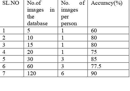
[image:10.612.86.304.216.369.2]The tabulated results were taken by considering the factors such as total number of images,number of images per person against accuracy for two test images with varying expressions.
Table 1. Accuracy Of PCA
SL.NO No.of
images in the
database
No. of
images per person
Accuracy(%)
1 5 1 60
2 10 1 80
3 15 1 80
4 20 1 75
5 30 3 85
6 60 3 77.5
7 120 6 90
Graphical User Interface
To enhance the usability of the program a GUI has been created which has push buttons to display the mean image,eigen faces,train and test the system and a text box displays the final result.This helps the user to easily understand and use the system.
15 LIMITATIONS OF THE ALGORITHM
Success of a practical face recognition system with images grabbed live depends on its robustness against the inadvertent and inevitable data variations. Specifically, the important issues involved are:
• Facial size normalization
• Non-frontal view of the face (3D pose,
head movement)
• Tolerance to facial expression /
appearance (including facial,hair & specs)
• Invariance to lighting conditions
(including indoor / outdoor)
• Facial occlusion (sunglasses, hat, scarf,
etc.)
• Invariance to aging.
We tried to minimize the data variations by capturing the facial image subjected to the reasonably constrained environment –
• Frontal view geometry and
• Controlled lighting.
16. FUTURE SCOPE:
This project is based on eigenface approach that gives a maximum accuracy the images are taken in constrained environment.Adaptive algorithms may be used to obtain an optimum threshold value. There is scope for future betterment of the algorithm by using Neural Network technique that can give better results as compared to eigenface approach. With the help of neural network technique accuracy can be improved.
Instead of having a constant threshold, it could be made adaptive,depending upon the
conditions and the database available, so as to maximise the accuracy.The whole software is dependent on the database and the database is dependent on resolution of camera. So if good resolution digital camera or good resolution analog camera is used , the results could be considerably improved.
17. CONCLUSION
Many methods of making computers recognize faces were limited by the use of improvished face models and feature descriptions(matching simple distances), assuming that a face is no more than the sum of its parts,the individual features. They tend to hide much of the pertinent information in the weights that makes it difficult to modify and valuate parts of the approach.
ISSN: 1992-8645 www.jatit.org E-ISSN: 1817-3195 best approximates the set of known face
images,without regarding that they correspond to our intutive notions of facial parts and features.
The eigenface approach provides a practical solution that is well fitted for the problem of face recognition. (1) It is fast, relatively simple, and works well in a constrained environment.Certain issues of robustness to changes in lighting, head size, and head orientation , the tradeoffs between
the number of eigenfaces necessary for
unambiguous classification are matter of concern.
REFERENCES
[1].Prof. Y. Vijaya Lata1, Chandra Kiran Bharadwaj Tungathurthi2, H. Ram Mohan Rao3, Dr. A. Govardhan4, Dr. L. P. Reddy ,” Facial Recognition using Eigenfaces by PCA”, International Journal of Recent Trends in Engineering, Vol. 1, No. 1, May 2009. [2].http://www.ces.clemson.edu/~stb/ece847/fall20
04/projects/proj13.doc
[3].http://afitsfacetag.site50.net/docs/AFITS_MidR eview.pdf
[4].http://en.wikipedia.org/wiki/Eigenvalue,_eigen vector_and_eigenspace
[5].http://en.scientificcommons.org/45529954 [6].http://www.ilkeratalay.com/download/eigenfac
es_msc_thesis.pdf
[7].Bruce Poon,M.Ashraful Amin,Hong Yan,”PCA
BASED FACE RECOGNITION AND
TESTING CRITERIA”,proceedings of
Eighth International Conference on Machine
Learning and Cybernetics,Baoding,12-15
July 2009.
[8].D. Pissarenko “Eigenface-based facial
recognition” Voil 1 No.3, 2003. pp 4-9. [9] M. Turk and A. Pentland, “Eigenfaces for
Recognition”, Journal of
CognitiveNeuroscience, vol.13, no. 1, 71-86, 1991.
[10].M.A. Turk and A.P. Pentland. “Face
recognition using eigenfaces”. In Proc. of Computer Vision and Pattern Recognition, pages 586-591. IEEE June 1991b.