NEW MODEL TRANSFORMATION USING REQUIREMENT TRACEBILITY FROM REQUIREMENT TO UML BEHAVIORAL DESIGN

PREDICTION OF RESEARCH TOPICS USING

COMBINATION OF MACHINE LEARNING AND LOGISTIC

CURVE

1

AGUS WIDODO, 2NOVITASARI NAOMI, 3SUHARJITO, 4FREDY PURNOMO

1

Lecturer, Faculty of Computer Science, Bina Nusantara University, Indonesia

2

Graduate Student, Faculty of Computer Science, Bina Nusantara University, Indonesia

3

Head of Graduate Program on Information Technology, Bina Nusantara University, Indonesia

4

Head of School of Computer Science, Bina Nusantara University, Indonesia

E-mail: 1aguswdd@yahoo.com, 2novitanaomi11@yahoo.com, 3suharjito@binus.edu,

4

fpurnomo@binus.edu

ABSTRACT

Prediction of future research topics is usually undertaken, especially by policy makers in research environment, to determine the focus of future studies. Analysis of future research topics by using a numerical approach based on scientific publications or patents have been previously done by several researchers mostly by classifying the topics based on the similarity of the documents. Meanwhile, time series analysis using statistical techniques, machine learning and logistic curves has also been conducted but for areas other than research topics. In this study, we will perform time series analysis to predict the topic of research by employing combination of machine learning approaches such as Neural Network, Extreme Learning Machine and Support Vector Machine. The prediction result is then finally refined by logistic curve. The dataset used in this study is a research report on Bioinformatics from Microsoft Research and NCBI (National Center for Biotechnology Information), over the past 30 years. Experimental result indicates that the combination of machine learning approaches and logistic-curve may improve the prediction accuracy. In addition, the emerging topic of the same dataset can be predicted with a relatively high average precision. Based on the dataset used, some emerging topics predicted for the next three years are 'Sequence Alignment', 'Index Terms', 'Secondary Structure', 'Nucleic Acid', and 'Saccharomyces cerevisiae'.

Keywords: research topics, prediction, bioinformatics, combination, machine learning, logistic curve

1. INTRODUCTION

Researchers and policy makers need to understand the current and future state of research, and be able to identify areas of research that has great potential. Meanwhile, the information sources of research today have grown rapidly along with the advancement of the internet. Meanwhile, the ways to predict the future topics of research, in general can be categorized into judgmental and quantitative analysis [1]. Predictions based on numerical data extrapolate historical data through a specific function, whereas the judgmental forecasting can also be based on projections from the past, but the sources of information in the model depend on the subjective judgments of experts. It is stated in [2] stated that the forecasting analysis through Delphi study by panel of experts is partially incompatible with the results of numerical analysis, since the

representation of experts in the panel, which cannot always be proportional, would impact the prediction accuracy.

Trend analysis of research topic by using a numerical approach based on scientific publications and / or patents have been done in some previous researchers, for example, Small [3], Rahayu and Hasibuan [4], Daim [5], Woon, Hensche and Madnick [6] , Ziegler [7], as well as Vidican et al.[8]. Those researchers calculate the same word in a document to group the documents into a certain category, and calculate the frequency of words to determine its trends.

and machine learning techniques to the data of a patent. In out previous research [11], we use time series analysis to make predictions on data from PubMed, and reveal that machine learning techniques can provide better performance than statistical approaches. Meanwhile, the ensemble between the logistic curve and statistical techniques (ARIMA) is done by Christodulous et al. [12] to make predictions with limited data.

Meanwhile, recently, much attention have been given to the kernel learning which tries to minimize both the error (loss function) in classification or regression and the coefficient of linear combination of kernels during the training [13, 14]. Thus, in this study, we will perform time series analysis to predict the topic of research by combining the recent machine learning techniques, namely the Multi Kernel Learning (MKL) and the logistic curve. The use of MKL is based on the advantages of this technique in the automatic selection of kernel, while the use of the logistic curve is based on the assumption that the research topics that have a limitation (capacity) in its growth cycle.

The rest of this paper is organized as follows. In section 2 we review some related works on time series prediction on research topics, in section 3 we present theoretical background of MKL and growth curve, in section 4 we describe the experimental setup including the steps taken, dataset and tools used, in section 5 we discuss our findings, and in section 6 we draw our conclusion.

2. RELATED WORKS

2.1 Prediction on Research Topics

Studies on the topic of research have been conducted by several researchers previously. Small [3] using co-citation clustering area for research in the field of science, while Rahayu and Hasibuan [4] and Zhu et al. [20] used co-word analysis. To determine the categories of research topics that are growing, Rahayu and Hasibuan [4] use a certain percentage limit, such as between one to three percent of the total number of patents or scientific publications.

Woon et al. [6] conducted a study on technology trends using bibliometrics, namely the number of records generated from a query against the database online. From the titles and abstracts obtained, derived keywords (terms) are then arranged in a taxonomy by using the Normalized Google Distance. Technology growth scores are calculated based on the average year of publication (average

publication year), the term frequency multiplied by the year divided by the frequency of the term during the observation period. Thus, the last year will provide a greater impact on the size of the growth.

Previously, Kobayashi et al. [15] make predictions of specific technology by using online information. Terms in the dictionary is used to filter the keywords obtained from the search results. In [15], techniques are used to combine similar keywords, to determine the hierarchy between the keywords and to determine the importance of a keyword.

2.2 The Use of Logistic Curve

There are several studies that use logistic curve to predict future technology trends. Christodoulos et al. [12] combines statistical methods, namely ARIMA (Autoregressive Integrated Moving Average) with a logistic curve to predict the level of technology diffusion. These two approaches are developed in a different research perspective and phenomenon. Diffusion model is derived from the biological sciences, industrial economics and business economics. On the other hand, the ARIMA model is derived from mathematics or statistics, which is typically used for prediction after obtaining a considerable amount of data. Study in [12] indicates that ARIMA method is better for short-term prediction, while the logistic curve is better for long-term prediction. ARIMA prediction results are used as the actual data to build models of diffusion. The authors concluded that the combination of the two approaches produced better performance than individual predictor.

Daim et al. [5] make predictions in three areas of technology to integrate the use of bibliometrics and patent analysis in technological forecasting techniques, namely the planning scenario, the growth curve (S-curve) and analogy. Data sources are grouped into several R & D categories, such as the Science Citation Index for basic research, the Engineering Index for applied research, U.S. Patent for the development phase, Abstract Daily Newspaper for the application phase and the Business and Popular Press for social impact.

technologies that are correctly predicted by experts with the Delphi method are in the growing stage, but others are actually in a relatively idle phase.

3. THEORETICAL BACKGROUND

3.1. Machine Learning for prediction

Three well known machine learning techniques for prediction are used in this paper, namely Artificial Neural Network, Support Vector Machine for Regression and Extreme Learning Machine.

Neural Network is well researched regarding their properties and their ability in time series prediction. Data are presented to the network as a sliding window [22] over the time series history, as shown in Figure 1. The neural network will learn the data during the training to produce valid forecasts when new data are presented.

Fig. 1 Predicting future value using Neural Network

The general function of NN, as stated in [22] is as follows:

(1) where X =[x0, x1, ..., xn] is the vector of the

lagged observations of the time series and w=(β, γ) are the weights. I and H are the number of input and hidden units in the network and g(.) is a non-linear transfer function. Default setting from Matlab is used in this experiment, that is 'tansig' for hidden layers, and 'purelin' for output layer, since this functions are suitable for problems in regression that predict continuous values.

Meanwhile, Support Vector Regression (SVR) is a Support vector machines (SVM) for regression which represents function as part of training data, often called as support vectors. Muller et al. [21] stated that SVM deliver very good performance for time series prediction. Given training data {(x1, y1),

K, (x1, y1)}⊂ X×R, where X is the input pattern,

SVM would seek function f(x) that has maximum deviation ε from target value yi. A linear function f

can be written as

with w∈X , b∈R (2) A flat function can be achieved by finding small

w by minimizing norm, . Technique

which enable SVM to perform complex nonlinear approximation is by mapping the original input space into the higher dimensional space through a mapping Φ, at which each data training xi is

replaced by Φ(xi). The explicit form of Φ does not

need to be known, as it is enough to know inner product in the feature space, which is called the kernel function, K(x,y) = Φ(x)⋅Φ(y).

In addition, Extreme Learning Machine is actually a feedforward neural network with one hidden layer, or better known as single hidden layer feedforward neural network. ELM has several interesting and significant features different from traditional popular gradient-based learning algorithms for feedforward neural networks [24], such as (1) the learning speed of ELM is extremely fast, (2) ELM has better generalization performance than the gradient-based learning such as backpropagation in most cases, (3) ELM tends to reach the solutions straightforward without issues like local minima, improper learning rate and over fitting, (4) ELM learning algorithm could be used to train SLFNs with many non differentiable activation functions.

ELM having N hidden nodes and activation function g(x) can be describes mathematically as follows:

(3) where wi is the weight vector which connect the

ithhidden node and input node, βi is the merupakan

weight vector which connects the ith hidden node and the output node, bi is the threshold of ithhidden

node, and wixj is the inner product of dari wi and xj.

Furthermore, the equation can be simplified into

, where the output weight connected to the

hidden layer can be computed as: ,

assuming that the input and its bias are determined randomly.

3.2 Logistic curve

Logistic curve method, which is usually called the S-curve or growth curve, assumes that the growth usually has shape like a letter S, which can be further divided into three stages. The first is a slow initial growth, followed by a period of rapid growth and ultimately a saturation phase in the upper slope. Mathematical function or a model is usually used for this extrapolation. Logistic curve which is used in modeling the growth of biological species in [17] can be formulated as:

X(t)

Hidden units X(t-1)

X(t-2)

X(t+1)

...

(4)

where K is the upper limit or carrying capacity of a particular technology, r is the initial rate of growth velocity, and t0 is the initial time of growth. K value is usually obtained from secondary data or expert opinion. If the upper limit value of K is unknown, it can be estimated by minimizing the sum of squared error is:

(5)

3.3 Growth rate

In [6, 7], several alternatives are devised to calculate the growth rate of a research topic, namely (1) the difference between the frequencies in the last year and early years, (2) the ratio between the frequency in the last year and early years, (3) the fitting of an exponential curve, and (4) the average year of publication. To provide a more balanced result, then the frequency of certain terms can be normalized by dividing these frequencies by the total number of publications in a given year. Fitting of an exponential curve will result in the form of , where r is a measure of growth rate. While the average of publication year is calculated by adding up years of the publication of results between years and the multiplication in the frequency divided by the total number of frequencies, such as

(6)

Thus, the publication last year will have a weight higher than previous years.

4. EXPERIMENTAL SETUP

4.1. Methodology

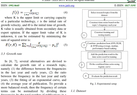
The steps to conduct experiments, as shown in Figure 2, are: (1) selecting the research topics, constructing the time series and building matrices for training and testing, (2) running the machine learning predictors, such as Neural Network, Extreme Learning Machine and Support Vector Regression with several different parameters (3) fitting the results of forecasting using the logistic curve, and (4) evaluating the performance of prediction.

Construct time series based on the topic’s frequency each year

Construct training and testing matrix

Add the prediction result to the time series used for training

Fit the combined time series using logistic curve

Combine prediction from ANN, ELM, & SVM using average, median,

performance based ranking Select research topics from the

dataset

3 1

2

Evaluate the prediction result

4

Fig. 2. Experimental setup

1.1.Dataset

The dataset is derived from research report on Bioinformatics from Microsoft Academic Research and NCBI (National Center for Biotechnology Information). Data sources from the scientific journals Microsoft Academic Search starts from 1963 to 2011. The number of publications will be grouped based on 50 keywords popular today, such as Gene Expression, Protein Sequence, Gene Expression Data, Phylogenetic Tree, Microarray Data, Large Scale, High Throughput, Dna Microarray, DNA Sequence, Support Vector Machine, Genetics, Sequence Alignment, etc. The number of journals will be obtained by utilizing the features of the top keywords on the Microsoft Academic Search, which can be accessed through http://academic.research.microsoft.com. In this site, we can find the number of publications per year and its citation.

For experimental purpose, we combine both data since they have keywords in common. Total keywords us is 20 based on the highest frequency of those keywords. The length of prediction is 3 years ahead. One of the time series is shown in Figure 3.

0 5 10 15 20 25 30 35

0 0.1 0.2 0.3 0.4 0.5 0.6 0.7 0.8 0.9 1

Fig. 3. One of the time series of topic ‘Expression Pattern’

The number of samples to be used as a training and testing is influenced by the length of time series. If there are k values to predict, the ytest

vector will contain k values, and xtest matrix will consist of m × k, where m is the sliding window. Thus, having 3 values to predict, the vector ytest

consists of 3 values, and the matrix xtest consists of

m×3 series, where m is the sliding window. The value of m is determined while constructing the training dataset, namely the xtrain and ytrain, whose

matrix’s size are m×n and n. The shorter the value of m the larger the dataset (which is n) that can be constructed, and vice versa. The example of xtrain as

a sliding window is shown in Figure 4.

-1.1 -1 -0.9 -0.8 -0.7 -0.6 -0.5 -0.4 -0.3

1 2 3 4 5 6

N

or

m

al

iz

ed

fr

eq

ue

nc

y

Time scale

sliding window1 sliding window2 sliding window3

Fig. 4. Example of sliding window of training data

1.2.Performance Evaluation

To evaluate performance, calculated Mean Squared Error (MSE) of the data out-of-sample, the data is not used in training. MSE is the difference between the estimated and actual values. If X = {x1,

x2, .. xt} is an input vector in the domain of f, and

the actual value is Y = {y1, y2, .. yt} is to sample as many as N, the error rate is calculated by

(7) where yi is the actual value and f(xi) is the

forecast value.

Another measure that is often used in previous papers is the mean absolute percentage error (MAPE). MAPE is a measure of accuracy of a method for constructing fitted time series values in statistics, specifically in trend estimation. It usually expresses accuracy as a percentage, and is defined by the formula:

(8)

In addition, to measure the ranking performance of the most emerging trends, the average precision is used. In the field of information retrieval, precision is the fraction of retrieved documents that are relevant to the search:

1.3.Hardware and Tools

This experiment is conducted on computer with Pentium processor Core i3 and memory of 4GB. The main software used is Matlab version 2008b. The NN code is provided by Matlab itself, while ELM is provided by Huang [24], and SVR is provided by Gunn [23].

5. RESULT AND DISCUSSION

5.1 Prediction Performance

Table 1. Performance of individual ANN, MKL and SVR

ts1 ts2 ts3 … ts20 Avg

NN hn=1 0.00 0.00 0.04 0.05 6.56

NN hn=2 0.00 0.01 0.05 0.01 23.87

NN hn=5 0.00 0.05 0.06 0.09 2.23

ELM hn=1 0.00 0.04 0.04 0.01 6.87

ELM hn=2 0.00 0.04 0.05 0.02 0.57

ELM hn=5 0.00 0.02 0.07 0.03 2.4E5

SVR RBF=0.5 0.00 0.00 0.00 0.01 0.26

SVR RBF=1 0.00 0.13 0.05 0.03 0.10

SVR RBF=2 0.00 0.04 0.02 0.02 1.78

SVR RBF=5 0.00 0.02 0.03 0.04 1.30

Tabel 1 Performance of combination of best models

avg median inv-mse rank

best model=1 23.87 23.87 23.87 23.87

best model=2 8.48 8.48 0.53 4.23

best model=3 2.69 0.25 1.06 0.59

best model=4 1.84 0.26 0.74 0.29

best model=5 2.41 0.49 0.74 0.37

best model=6 2.14 0.74 0.73 0.39

best model=7 1.63 0.39 0.13 0.38

best model=8 1.24 0.22 0.29 0.34

best model=9 1.03 0.10 0.27 0.32

best model=10 2405.73 0.11 0.27 278.99

Average 245.11 3.49 2.86 30.98

Of those three predictors with several different parameters, the performance results of combination through an average, weighted based on performance, and ranking are as shown in Table 3. The test is done using the best model selection, assuming that the best model on the validation data will yield good results on data testing. From the table it appears that the worst predictor will not get a high weight, so that the average MSE (mean squared error) of the combined prediction is much better than the average individual prediction. So there is improvement in the rankings with the use of S-Curve (logistic curve) to calibrate the predicted results.

Fig. 5. Illustration of performance of combination of methods

Figure 5 further illustrates the performance of the method of the combination, which may be

concluded that a good performance can be achieved with a number of the best models from 3 to 9 from a total of 10 models, or the lowest MSE can be seen in the figure at around 40% of the total number of models.

5.2 Emerging research topics

To find a research topic that has considerable potential, or so-called emerging, equation from Ziegler [7] which puts more weight on current year is used. Table 3 shows the first ten of the most emerging topics out of 20 topics from the prediction and from the actual time series. Using the average precision, the ranking performance of the emerging topics is 0.95.

Tabel 3. The first ten most emerging topics

Rank Existing Data Prediction

Preci-sion

1 'Secondary Structure' 'Secondary Structure' 1

2 'Nucleic Acid'

'saccharomyces

cerevisiae' 0.5

3

'saccharomyces

cerevisiae' 'Nucleic Acid' 1

4 'Dna Sequence' 'Dna Sequence' 1

5 'Amino Acid' 'Amino Acid' 1

6 'Nucleotides' 'Nucleotides' 1

7 'Binding Site' 'Binding Site' 1

8 'High Throughput' 'High Throughput' 1

9 'Large Scale' 'Large Scale' 1

10 'Indexing Terms'

'Statistical

Significance' 0.9

Furthermore, to determine the potential topics in the future, such as 3 years ahead, the developed techniques can generate emerging topics such as shown on the table below.

Table 5. Prediction of 10 emerging topics for 3 years ahead

Rank Prediction Result Score

1 'Sequence Alignment' 2372.146

2 'Indexing Terms' 2063.848

3 'Secondary Structure' 2053.827

4 'Nucleic Acid' 2050.084

5 'saccharomyces cerevisiae' 2027.9

6 'Dna Sequence' 2020.467

7 'Amino Acid' 2015.151

8 'Nucleotides' 2014.271

9 'Binding Site' 2013.706

10 'Protein Structure' 1985.395

6. CONCLUSION

with the machine learning method for data that has properties of growth-curve to yield better prediction accuracy compared to the average of individual predictors or the combination of machine learning predictors without the growth-curve. In addition, based on the available dataset, this experiment projects several topics that are emerging in the years ahead, such as 'Sequence Alignment', 'Indexing Terms', 'Secondary Structure', 'Nucleic Acid', and 'saccharomyces cerevisiae'.

However, more diverse and longer time span dataset is needed to further confirm this hypothesis. In addition, this dataset has a fairly large fluctuation that is relatively more difficult to detect its pattern. For further research, it is also worth to try other mechanisms in combining the prediction, either combining the results or combining the kernel of individual predictors.

REFERENCES:

[1] J.R. Meredith, S.J. Mantel, Technological Forecasting, John Wiley & Sons, Inc., 1995. [2] M. Bengisu, R. Nekhili. “Forecasting emerging

technologies with the aid of science and technology databases”. Technological

Forecasting & Social Change 2006; 73: 835–

844.

[3] H. Small, “Tracking and predicting growth areas in science”. Scientometrics, 2006, 68(3):595–610.

[4] E.R. Rahayu, and Z.A. Hasibuan, “Identification of technology trend on Indonesian patent documents and research reports on chemistry and metallurgy fields”.

Proceeding Asia Pacific Conf., Singapore,

2006.

[5] T.U. Daim, G. Rueda, H. Martin, and P. Gerdsri, “Forecasting emerging technologies: Use of bibliometrics and patent analysis”.

Technological Forecasting and Social

Change, October 2006, 73(8):981–1012.

[6] W.L. Woon, A Hensche, and S Madnick, “A Framework For Technology Forecasting And Visualization”. Working Paper Series, ESD-WP-2009-16, October 2009.

[7] B.E. Ziegler. “Methods for Bibliometric Analysis of Research: Renewable Energy Case Study”. Working Paper CISL#2009-10, September 2009.

[8] G. Vidican, W.L. Woon, S. Madnick. “Measuring Innovation Using Bibliometric Techniques: The Case of Solar Photovoltaic

Industry”, Working Paper CISL# 2009-05, 2009.

[9] N. R., Smalheiser. “Predicting emerging technologies with the aid of text-based data mining: the micro approach”, Technovation, 21(10):689–693, October 2001.

[10] S. Jun, D. Uhm. “Technology Forecasting Using Frequency Time Series Model: Bio-Technology Patent Analysis”. Journal of

Modern Mathematics & Statistics, 2010,

4(3):101-104.

[11] A. Widodo., M.I. Fanany, I. Budi. “Technology Forecasting in the Field of Apnea from Online Publications: Time Series Analysis on Latent Semantic”. International Conference on Digital Information

Management, 26-28 September 2011,

Melbourne, Australia.

[12] C. Christodoulos, C. Michalakelis, D. Varoutas. “Forecasting with limited data: Combining ARIMA and diffusion models”. Technological Forecasting & Social Change 2010, 77: 558–565.

[13] A. Rakotomamonjay, F Bach, S Canu, Y Grandvalet. “SimpleMKL”, Journal of

Machine Learning Research X, 2008, pp.

1-34.

[14] M. Varma, and B.R. Babu, “More generality in efficient multiple kernel learning”. In

Proceedings of the International Conference

on Machine Learning, 2009.

[15] S. Kobayashi, Y. Shirai, K. Hiyane, F. Kumeno, H. Inujima. “Technology Trends Analysis from the Internet Resources”.

PAKDD 2005, LNAI 3518, Springer-Verlag

Berlin Heidelberg, 2005, pp. 820–825, 2005. [16] B. Scholkopf, A. Smola, Learning with

Kernels, The MIT Press, 2001.

[17] J.H. Mathews. Bounded Population Growth: A

Curve Fitting Lesson. Mathematics and

Computer Education, California State Univ, 1992.

[18] R. Polikar. “Ensemble Based System in Decision Making”, IEEE Circuits And

Systems Magazine, 2006, vol. 6, pp. 21-45.

[19] J. Shawe-Taylor and N. Cristianini, Kernel

Methods for Pattern Analysis, Cambridge

University Press, 2004.

Center, Georgia Institute of Technology, Atlanta, GA, 1998.

[21] K. R. Muller, A. J. Smola, G. Ratsch, B. Scholkopf, J. Kohlmorgen, and V. Vapnik “Predicting Time Series with Support Vector Machines”, Proceedings of the 7th International Conference on Artificial Neural Networks, Springer-Verlag London, UK, 1997.

[22] N. Mirarmandehi, M. M. Saboorian, A. Ghodrati, “Time Series Prediction using Neural Network”, 2004.

[23] S. R. Gunn, “Support Vector Machines for Classification and Regression”, Technical Report, University Of Southampton, 10 May 1998.