A Note on Parameterized Preconditioned Method for Singular Saddle Point Problems

http://dx.doi.org/10.4236/jamp.2016.44067

How to cite this paper: Lv, Y.Y. and Zhang, N.M. (2016) A Note on Parameterized Preconditioned Method for Singular Sad-dle Point Problems. Journal of Applied Mathematics and Physics, 4, 608-613. http://dx.doi.org/10.4236/jamp.2016.44067

A Note on Parameterized Preconditioned

Method for Singular Saddle Point Problems

Yueyan Lv, Naimin Zhang

*

School of Mathematics and Information Science, Wenzhou University, Wenzhou, China

Received 3 December 2015; accepted 6 April 2016; published 13 April 2016

Abstract

Recently, some authors (Li, Yang and Wu, 2014) studied the parameterized preconditioned HSS (PPHSS) method for solving saddle point problems. In this short note, we further discuss the PPHSS method for solving singular saddle point problems. We prove the semi-convergence of the PPHSS method under some conditions. Numerical experiments are given to illustrate the efficien-cy of the method with appropriate parameters.

Keywords

Singular Saddle Point Problems, Hermitian and Skew-Hermitian Splitting, Preconditioning, Iteration Methods, Semi-Convergence

1. Introduction

We consider the iterative solution of the following linear system:

* 0

B E y f

Ax b

E z g

     =_{    }= ≡

−

     (1)

where p p

B∈C × is Hermitian positive definite, p q

E∈C × is rank-deficient, i.e., p≥q, *

E denotes the conjugate transpose of E, p

f∈C and q

g∈C . Linear systems of the form (1) are called saddle point prob-lems. They arise in many application areas, including computational fluid dynamics, constrained optimization and weighted least-squares problem, see, e.g., [1] [2].

We review the Hermitian and skew-Hermitian splitting (HSS) [3] of coefficient matrix A:

A=H+S

where

(

*

)

0

1

0 0

2

B

H= A+A =  _

 ,

*

* 0 1

( )

0 2

E

S A A

E

 

= − _{=  }

−

 .

The PPHSS Iteration Method ([4]): Denote n= +p q. Let (0) n

x ∈C be an arbitrary initial guess, com-*_{Corresponding author. This author is supported by National Natural Science Foundation of China under grant No. 61572018 and Zhejiang}

pute (k 1)

x + for k=0,1, 2,... by the following iteration scheme until ( )

{xk} converges,

( 1/2) ( )

( 1) ( 1/2)

( ) ( )

.

( ) ( )

k k

k k

P H x P S x b

P S x P H x b

α α

β β

+

+ +

 + = − +



+ = − +

 (2)

where α, β are given positive constants and

0

0

B P

C

 

=  

  (3)

matrix C is Hermitian positive definite.

Evidently, the iteration scheme (2) of PPHSS method can be rewritten as

(k 1) _{( , )} ( )k _{( , )}

x + =T α β x +F α β b (4)

here, T( , )α β is the iteration matrix of the PPHSS method. In fact, Equation (4) may also result from the split-ting

( , ) ( , )

A=M α β −N α β (5) with

1

*

( 1) ( 1)

1 1

( , ) ( )( ) B E

M P P H P S

E C

β α α

α β α β

α αβ

α β − α β

+ +

 

= + + = _{ }

−

+ _{+  } (6)

Evidently, the matrix M( , )α β can act as a preconditioner for solving the linear system (1), which is called the PPHSS preconditioner. The PPHSS method is a special case of the generalized preconditioned HSS (GHSS) method [5]. When β α α= / ( +1), we can obtain a special case of the PPHSS (SPPHSS) method. In order to analyze the semi-convergence of the PPHSS iteration, we let

1/2 1/2 1/2 1/2

* 0 0

0 0 ₀

P E

I

H P HP S P SP

E

− −   − − _ _

= =_{ } = =

 

 ， _− _

where I _p is the identity matrix of order p and E=B−1/2EC−1/2. In the same way, we denote

1/2 1 1/2

( , ) ( , ) ( , )

T α β =P M α β − N α β P− (7)

Owing to the similarity of the matrices T( , )α β and T( , )α β , we only need to study the spectral properties of matrix T( , )α β in order to analyze the semi-convergence of the PPHSS iteration.

2. The Semi-Convergence of the PPHSS Method

As the coefficient matrix A is singular, then the iteration matrix T has eigenvalue 1, and the spectral radius of matrix T cannot be small than 1. For the iteration matrix T of the singular linear systems, we introduce its pseu-do-spectral radius ν( )T by follows,

{

}

( )T max | |: ( ),T 1

ν = λ λ σ∈ λ≠ ,

where σ(T) is the set of eigenvalues of T.

For a matrix K∈Rn×n, the smallest nonnegative integer i such that rank K( i)=rank K( i+1) is called the index of K, and we denote it by i=index K( ). In fact, index K( ) is the size of the largest Jordan block corres-ponding to the zero eigenvalue of K.

Lemma 2.1 ([6]). The iterative method (4) is semi-convergent, if and only if,

( ( , )) 1

index I−T α β = and ν( ( , ))T α β <1.

Lemma 2.2 ([7]). index I( −T( , ))α β =1, if and only if, for any 0≠ ∈Y R A( ), Y∉N AM( −1).

Theorem 2.3. Assume that B and C be Hermitian positive definite, E be of rank-deficient. Then ( ( , )) 1

index I−T α β = .

Lemma 2.4 ([4]). Let B and C be Hermitian positive definite, E be of rank-deficient. Assume that

' 1 *

q

S βI E E

β

= + . Then, we can partition T( , )α β in Equation (7) as

1 1

2

1 1

( 1) ( )( )

( 1) ( 1) 1

( )( ) 1 ( )

( 1) 1 1

*

' '

p

*

' '

q

α β _I α β αβ β α _{E S E} α β_{E S}

β α αβ α α

T

α β αβ β α β β α β

S E I S

αβ α α α

− −

− −

− + + − +

 _{− −} 

 _{+ + +} 

 

=

 + + − − + 

+

 _{+ + +} 

 

.

Let E=U*Σ'V be the singular value decomposition [9] of E, where U∈Cp p× and V∈Cq q× are unitary matrices, and

'

1 2 ( , ,..., ) 0

q q q

diagσ σ σ C ×

 Σ

Σ =  Σ = ∈

 ， ,

( 1, 2,..., )

i i q

σ = are the singular values of E.

Lemma 2.5. The eigenvalues of the iteration matrix T( , )α β of PPHSS iteration method are ( 1) ( 1)

α β

β α

− +

with multiplicity p−q, and the roots of quadratic equation

2 ₂ 2

2

2 2

2 2

(2 )( ) ( 1)( )

0

( 1)( ) ( 1)( )

k k

k k

αβ β α αβ σ β β α σ

λ λ

α α β σ α α β σ

+ − − − +

− + =

+ + + + , k=1, 2,...,q (8)

Proof. Notice the similarity of matrices T( , )α β and T( , )α β . The proof is essentially analogous to the proof of Lemma 2.3 in [4] with only technical modifications. So, it is omitted.

Lemma 2.6. If σ ≠k 0, then the eigenvalue λ of the iteration matrix T( , )α β satisfies λ≠1; if σ =k 0, then λ=1 or ( 1)

( 1)

α β

β α

−

+ .

Proof. If σ ≠k 0, we give the proof by contradiction. By Lemma 2.5, obviously, when

( 1) ( 1)

α β λ

β α − =

+ , it can

not be equal to 1. We assume λ± =1, by some algebra, it can be reduced to

2

2 2 2 2

(2α 2αβ α β σ) k (α β αβ ) dk 4ek 0

− + + + − + ± − = ,

here, d_k =(2αβ β α αβ σ+ − )( − 2k) and

2 2

2 2

( 1)( 1)( k)( k)

k

e =αβ α+ β− α +σ β +σ . It is equivalent to

2 ₂ 2

( ) 0

k k

σ β +σ = , so σ =k 0, which is in contradiction with σ ≠k 0.

If σ =k 0, we have λ₊=1 and

( 1) ( 1)

α β

λ

β α

−

− =

+ , which finishes the proof.

Lemma 2.7 ([10]). Both roots of the real quadratic equation are less than one in modulus if and only if | | 1c<

and | | 1b< +c.

Theorem 2.8. If the iteration parameters α and β

2 1

α _{β α}

α+ < ≤ , α >0 (9)

then, the pseudo-spectral radius of the PPHSS method satisfies ν( ( , ))T α β <1. Proof. Using condition (9), it follows that | 1 | 1

( 1)

α β

β α

− _<

+ . According to Lemma 2.5, if σ ≠k 0, we can obtain that

2 2

2 2

2 2

2 2

( 1)( ) | 1 | ( )

| | 1

( 1)( ) ( 1)( )

k k

k

k k

c β β α σ β β α σ

α α β σ α α β σ

− + − +

= = <

and

2 2

2 2

2 2

(2 )( ) (2 ) [ ( 1) ( 1)]

1

( 1)( ) ( 1)( )

k k

k k

k k

b αβ β α αβ σ αβ αβ β α α α β β σ c

α α β σ α α β σ

+ − + + − + + + −

< < = +

+ + + + .

By Lemma 2.7, for the eigenvalues λ of T( , )α β , it holds |λ <| 1. If σ =k 0, by Lemma 2.6, the eigenvalues of T( , )α β , except 1 are

( 1) ( 1)

α β

β α

−

+ . According to the definition

of pseudo-spectral, we get ν( ( , ))T α β <1.

Theorem 2.9. Let

σ

min =min_{1≤ ≤k q}{

σ σ

k: k ≠0} and

σ

max =max_{1≤ ≤k q}{

σ σ

k: k ≠0}. Then, the optimal value of the iteration parameter α for the SPPHSS iteration method is given by

2 2

*

min min min

0

1

arg min , 4

1 2

T α

α

α ν α σ σ σ

α >       ≡   _ ₊ _= _ + + _     , and correspondingly, * *

* _{2 2}

min min min

2 ,

1 _{2 4}

T α

ν α

α _{σ σ σ}

  

=

  

 _{ + }

  + + +

. (10)

Proof. According to Lemma 2.5 and Lemma 2.6, we know that the eigenvalues of the iteration matrix

( , )

T α β are 1 1

α

−

+ with multiplicity p, and 2 2 2 2 2 (1 ) k k α σ

α α σ

+

+ + , k=1, 2,..., .q (11)

If σ =k 0, the eigenvalues with the form of Equation (11) are 1, which can not affect the value of ( ( , ))T

ν α β . Therefore, without loss of generality, here we only need to discuss the case σ ≠k 0. The rest is similar to that of the proof of Theorem 3.1 in [4], here is omitted.

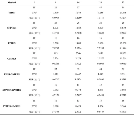
3. Numerical Results

In this section, we use an example to demonstrate the numerical results of the PPHSS method as a solver by comparing its iteration steps (IT), elapsed CPU time in seconds (CPU) and relative residual error (RES) with other methods. The iteration is terminated once the current iterate satisfies RES≤10−8 or the number of the prescribed iteration steps k=1, 000 are exceeded. All the computations are implemented in MATLAB on a PC computer with Intel (R) Celeron (R) CPU 1000M @ 1.80 GHz, and 2.00 GB memory.

Example 3.1 ([11]). Consider the saddle point problem (1), with the following block form of coefficient ma-trix: 2 2 2 2 0 0 l l

I L L I

B R

I L L I

× ⊗ + ⊗   =_{ }∈ ⊗ + ⊗   , 2 2

2 ( 2) 1 2

( ) l l

E E b b R

∧

× +

= ∈ ,

where symbol ⊗ denotes the Kronecker product, and

2 1

( 1, 2, 1) l l

L tridiag R

h

×

= ⋅ − − ∈ , E I Q R2l2 l2 Q I ∧ ⊗ ⊗   =_{ }∈ ⊗   , 2_/2 1 0 l e b E ∧  = _ _

 , 2

2 /2 0 l b E e ∧  = _ _  , 2 /2 2_/2 1,1,...,1 l

T l

e =（ ）∈R ,_Q 1 _tridiag( 1,1, 0) _Rl l

h

×

= ⋅ − ∈ , 1

1

h l

= + ,

the right-hand side vector b is chosen by b=Ae_{p q+} , where ep q (1,1,...,1)T Rp q

+

+ = ∈ , p=2l2, q= +l2 2.

For the Example 3.1, we choose T_ˆ 1

[image:5.595.87.536.101.256.2]

Table 1. The optimal iteration parameters and pseudo-spectral radius.

Method l 8 16 24 32

PHSS

*

α 1.6328 2.1999 2.6511 3.0367

* *

( (T , ))

ν α α 0.6756 0.8112 0.8667 0.8969

SPPHSS

*

α 1.0216 1.0059 1.0027 1.0015

* *

*

( ( , ))

1

T α

ν α

α + 0.4947 0.4985 0.4993 0.4996

PPHSS

exp

α 1.9815 2.6990 2.5976 2.9953

exp

β 0.6853 0.7845 1.0336 1.1234

exp exp

( (T , ))

ν α β 0.5209 0.5258 0.5340 0.5452

Table 2. IT, CPU and RES for T _ˆ 1

C=E B E− .

Method l 8 16 24 32

PHSS

IT 26 37 47 54

CPU 0.399 1.548 7.286 27.178

RES ( 9

10− ) 6.6914 7.2250 7.3711 9.3294

SPPHSS

IT 26 26 26 26

CPU 1.075 1.583 4.879 8.610

RES ( 9

10− ) 5.3781 6.7198 7.0689 7.2124

PPHSS

IT 16 16 16 16

CPU 0.220 1.008 3.620 12.558

RES ( 9

10− ) 7.8783 7.6704 7.7535 8.1446

GMRES

IT 883 2560 5450 10376

CPU 0.524 3.179 12.572 16.264

RES ( 9

10− ) 9.8243 9.9925 9.9903 9.9950

PHSS-GMRES

IT 22 35 44 50

CPU 0.111 0.467 1.649 3.751

RES ( 9

10− ) 9.6710 8.0874 9.3990 9.8588

SPPHSS-GMRES

IT 10 11 13 14

CPU 0.082 0.372 1.831 3.892

RES ( 9

10− ) 4.7178 6.7487 6.2498 4.2212

PPHSS-GMRES

IT 11 13 13 16

CPU 0.070 0.428 1.564 3.366

RES ( 9

10− ) 5.4534 2.3975 9.8449 9.8690

[image:5.595.90.538.288.672.2]

1 1 * 1 1 1

1

1 * 1 1

1

( )

( 1)

( , )

( 1)

B I ES E B B ES

M

S E B S

α β α β

β α β αβ

α β

α β α β

β α α

− − − − −

−

− − −

+ +

 _{− ′ − ′} 

 ₊ 

 

=

 + _′ + _′ 

 ₊ 

 

where S

β

C 1E B E* 1

β

−

′ = + . To compute the matrix-vector products with 1

( , )

M α β − , we make incomplete

LU factorization of B and S′ with drop tolerance 0.001. In the two tables, we use restarted GMRES (18) and preconditioned GMRES (18).

References

[1] Elman, H.C., Ramage, A. and Silvester, D.J. (2007) Algorithm 866, IFISS, a MatLab Toolbox for Modelling Imcom-pressible Flow. ACM Trans. Math. Softw., 33, 1-18.

[2] Bjorck, A. (1996) Numerical Methods for Least Squares Problems. SIAM, Philadelphia.

http://dx.doi.org/10.1137/1.9781611971484

[3] Bai, Z.Z., Golub, G.H. and Ng, M.K. (2003) Hermitian and Skew-Hermitian Splitting Methods for Non-Hermitian Positive Definite Linear Systems. SIAM J. Matrix Anal. Appl., 24, 603-626.

http://dx.doi.org/10.1137/S0895479801395458

[4] Li, X., Yang, A.L. and Wu, Y.J. (2014) Parameterized Preconditioned Hermitian and Skew-Hermitian Splitting Itera-tion Method for Saddle-Point Problems. Int. J. Comput. Math., 91, 1224-1238.

http://dx.doi.org/10.1080/00207160.2013.829216

[5] Chao, Z. and Zhang, N.M. (2014) A Generalized Preconditioned HSS Method for Singular Saddle Point Problems. Numer. Algorithms, 66, 203-221. http://dx.doi.org/10.1007/s11075-013-9730-y

[6] Berman, A. and Plemmons, R. (1979) Nonnegative Matrices in Mathematical Science. Academic Press, New York.

[7] Zhang, N.M. and Wei, Y.M. (2010) On the Convergence of General Stationary Iterative Methods for Range-Hermitian Singular Linear Systems. Numer. Linear Algebra Appl., 17, 139-154. http://dx.doi.org/10.1002/nla.663

[8] Chen, Y. and Zhang, N.M. (2014) A Note on the Generalization of Parameterized Inexact Uzawa Method for Singular Saddle Point Problems. Appl. Math. Comput., 325, 318-322. http://dx.doi.org/10.1016/j.amc.2014.02.089

[9] Golub, G.H. and Van Loan, C.F. (1996) Matrix Computions. 3rd Edition, The Johns Hopkins University Press, Balti-more.

[10] Young, D.M. (1971) Iterative Solution of Large Linear Systems. Academic Press, New York.