Performance Analysis of Floyd Warshall Algorithm vs Rectangular Algorithm

Performance Analysis of Floyd Warshall Algorithm vs

Rectangular Algorithm

Akanksha Singh

Department of Information Technology Birla Institute of Technology, Mesra (Ranchi) India

Pramod Kumar Mishra

ABSTRACT

In this paper, we have examined the comparative study of Floyd Warshall algorithm and the Rectangular algorithm. We have tested these two algorithms on random graphs generated by the Erdös – Renyi (ER) model. The evaluation of the algorithms for different probabilities show that the Floyd Warshall algorithm gives slightly better performance for dense graphs while the Rectangular algorithm works better for sparse graphs.

Keywords

Bellman ford algorithm, Dijkstra’s algorithm, Floyd warshall algorithm, all pair shortest path algorithm, the rectangular algorithm, comparison of algorithms.

1.

INTRODUCTION

The shortest path problem is a fundamental algorithmic problem, in which a minimum weight path is computed between two nodes of a weighted, directed graph. This problem has been studied for a long time and has attracted researchers from various areas of interests such as operations research, computer science, communication networks and VLSI design. Even after being a thoroughly explored problem, new developments keep emerging for this problem. The simple reason is that with new technological development. Its applications have also increased and require better performance than before. An efficient solution for this problem is needed by a variety of real-life applications like path finding in maps, robot navigation, urban traffic planning, optimal pipelining of VLSI chip, routing of telecommunication messages, network routing protocols and exploiting arbitrage opportunities in currency exchange. Also it is used as a subroutine in many advanced algorithms. In a shortest path problem, a graph G (V, E) is given, where, V is a set of n vertices and E is the set of m edges. Each edge connects two vertices and is associated with a weight. The weights can be positive or negative. The graph can be directed or undirected, may contain cycles or not. Most of the solutions to the shortest path problem assume that the graph doesn't contain any negative cycles. Various real life models can be represented as graphs, for example, in transport networks, roads represent edges and intersections represent vertices. The weights may be cost travelled along a road or time taken to travel that road, according to the situation.

There are mainly two versions of the shortest path problem:

 Single source shortest path problem (SSSP): Here, shortest paths from a source node to all other nodes of the graph are found.

 All pairs shortest path problem (APSP): Here, shortest paths for each pair of vertices in the graph are computed. This paper concentrates on the APSP problem, since most real life models need to evaluate the shortest paths for every pair

of vertices. In the next section, we discuss literature review where numerous researches done his works on the shortest path problem. In section 3, we explain performance analysis and comparative study of APSP algorithms. The experimental setup and results are described in sections 4 and 5 respectively. In section 6 we conclude the result.

2.

LITERATURE REVIEW

Being a classical problem, the shortest path problem has been investigated through various approaches. Many researchers formulate efficient algorithms for this problem. Some basic algorithms for evaluating shortest paths are explained below:

2.1

Bellman Ford Algorithm

This algorithm provides solution for the SSSP problem [1]. It is used for weighted, directed graphs which may have edges with negative weights, and has a time complexity of O (nm). It can also detect negative weight cycles in the graph.

2.2

Dijkstra's Algorithm

This algorithm also solves the SSSP problem, but it only works for graphs with nonnegative edge weights [2]. It has a running time of O (n2). If the min-priority queue used in Dijkstra's algorithm is implemented with a binary heap, the running time achieved is O (mlog (n)) [3]. By using Fibonacci heaps even better performance is obtained, that is, O (nlog(n) + m) [3].

2.3

Floyd Warshall algorithm

problem, along with optimization strategies for scale free complex networks.

2.4

All-Pairs Shortest Path Algorithms

Given is a weighted, directed graph G (V, E), where V is a set of n vertices and E is a set of m edges. It is represented by an adjacency matrix, whose elements are w[i, j], weight of the edge [i, j] for i, j = 1,2,...,n. These weights may be negative but the graph must not contain any negative cycle. For storing the weights of shortest paths, we have used a distance matrix having elements d[i, j] as the weight of shortest path from i to j, where i, j = 1,2,…,n. A predecessor matrix is used for constructing the shortest routes. Its elements are r[i, j], the

predecessor of j on the shortest path from i, where i, j = 1,2,...,n. We have to find the shortest paths between each

pair of vertices of the graph. The two algorithms we have used for comparison are explained below.

2.4.1

Floyd Warshall Algorithm

The Floyd Warshall algorithm is an elementary algorithm for finding out shortest paths for every pair of vertices in a directed graph. It is a dynamic programming algorithm. It was developed by Floyd [4] on the basis of a paper given by Warshall [14]. This algorithm is based on a concept of intermediate vertices. Let dij

0

be the weight matrix, and dij k

be the shortest path from i to j with its intermediate vertices in the set {1, 2... k}. Then for k > 1,

dijk = min( dijk-1 , dikk-1 + dkjk-1 ) (1)

Thus, dij n

will provide the shortest paths matrix for the input graph. The algorithm is stated below.

Algorithm 1

We have implemented the algorithm using single distance and predecessor matrices instead of using different matrices for each value of k. This is because if we were to compute and store dik or dkj before using these values to compute dij, we might be computing one of the following:

dijk = min( dijk-1 , dikk-1 + dkjk-1 ) (2)

dijk = min( dijk-1 , dikk + dkjk-1 ) (3)

dijk = min( dijk-1 , dikk-1 + dkjk) (4)

have to use different distance matrices for different values of k.

The time complexity of the algorithm is determined by the triple nested for loops that clearly show that the running time of this algorithm is Θ(n3). The distance matrix containing d[i, j] values provides the distance of shortest path from i to j and the route of the shortest paths can be easily constructed from the predecessor matrix containing r[i, j] values.

2.4.2

The Rectangular Algorithm

As given in [15], this algorithm is based on Floyd Warshall algorithm, and attempts to simplify it by a rectangular graphical approach. This approach reduces the computational effort of the algorithm and is easier to understand. Although it has the same time complexity as the Floyd Warshall algorithm.

Algorithm 2

Here, also we have used single distance and predecessor matrices, reason being the same as explained for the Floyd Warshall algorithm. The resulting distance matrix will contain the distances of shortest paths for each pair of vertices of the graph, and these routes can also be easily obtained from predecessor matrix.

For implementing this algorithm, we have used an extra array for remembering the indices of the rows and columns whose elements will not change according to step (a) of the algorithm. Then, for completing the distance matrix according to step (b), we will have triply nested for loops as in the Floyd Warshall algorithm, but we will skip the rows and columns whose indices we have stored initially. Thus, this algorithm uses an extra array which takes O(n) space.

3.

EXPERIMENTAL SETUP

1. for i = 1 to n do 2. for j = 1 to n do

3. if there exists an edge from i to j then

4. d[i, j] = w[i, j]

5. r[i, j] = i

6. else

7. d[i, j] = infinity

8. r[i, j] = -1

9. for k = 1 to n do 10. for i = 1 to n do

11. for j = 1 to n do

12. if d[i, k] + d[k, j] < d[i, j] then

13. d[i, j] = d[i, k] + d[k, j]

14. r[i, j] = k

1. for i = 1 to n do 2. for j=1 to n do

3. If there exists an edge from i to j then 4. d[i, j]=w[i, j]

5. r[i, j]= i 6. Else

7. d[i, j]=infinity 8. r[i, j]= -1 9. for k=1 to n do

10.a) If an Infinity exists in kth row or column of the distance matrix, the remaining entities of the row or column in which Infinity exists will not change. Thus, the d[i, j] values for the respective row or column will not change.

11.b) If applying rule (a) doesn't result in a complete distance matrix, then these remaining entities will be derived by drawing a set of rectangles, with dij, dik, dkj

and diagonal zero as the corners of the rectangle. 12.c) For the predecessor matrix, if d[i, j] value has not

model [16]. The ER model generates random graphs of n vertices where each possible edge can exist with probability p. The number of edges in the generated graph is a random variable with expected value pn(n-1)/2. Lower values of p imply sparse graphs and higher values imply dense graphs. Thus the parameters for the algorithms are n and p for which the running times of programs will be plotted. The running time has been averaged on 50 instances for each parameter setting. The average running times obtained have been plotted using Gnuplot (version 4.6.5).

We have first evaluated the performance of the algorithms on different values of p, keeping n = 100. Then we have compared the Floyd Warshall algorithm with the Rectangular algorithm, for p = 0.1, 0.3, 0.5 and 0.8, varying n from 10 to 100. In the next section, the results of the experiments are specified.

4.

PERFORMANCE ANALYSIS

4.1

Effects of Probability p

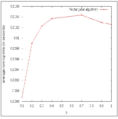
The performance of both the algorithms has been tested on different values of probability p. The plots for the Floyd Warshall algorithm and the Rectangular algorithm are given in figure 1 and 2 respectively.

Figure 1: Floyd Warshall Algorithm- Average Running Time VS Probability

As can be seen, the performance of Floyd Warshall algorithm improves with increasing value of p, but the change is very small in comparison to the running time. It means that the Floyd Warshall algorithm performs slightly better for dense graphs than sparse graphs.

In case of Rectangular algorithm, the average running time increases rapidly from p = 0.1 to p = 0.4, but for p > 0.4, there is not much change in the running time of the algorithm.

Figure 2: Floyd Rectangular Algorithm- Average Running Time VS Probability

So, the Rectangular algorithm provides better performance for sparse graphs.

4.2

Comparison of Algorithms

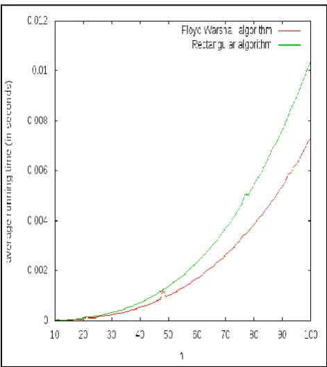
We have tested the two algorithms with number of nodes n varying from 10 to 100. The figures 3, 4, 5 and 6 plot the average running times of Floyd Warshall algorithm and Rectangular algorithm for p=0.1, 0.3, 0.5 and 0.8 respectively. As is visible from the graphs, the Rectangular algorithm's running time is higher than that for the Floyd Warshall algorithm. In case of p=0.1, the running times of both the algorithms is comparable for n < 60. For p = 0.3, 0.5, 0.8, both the algorithms have similar running times up to n = 30, but as n rises above 30, the difference starts escalating and the Floyd Warshall algorithm clearly performs better than the Rectangular algorithm.

This behaviour of the Rectangular algorithm can be explained by the fact that the section of the program that implements step (a) of the program slows down the program instead of speeding it up, especially for larger values of p. The step (a) of the Rectangular algorithm is supposed to increase its speed since it reduces the number of calculations required. But, the time spent in performing this step, that is, in remembering the indices of the rows and columns, whose elements will not change, is O (n). Thus, the time saved by doing less number of calculations is not enough to compensate for the time lost in the execution of step (a). Hence, both the algorithms have the same time complexity of Θ (n3

Figure 3: Floyd Warshall Algorithm VS Rectangular Algorithm (Probability p=0.1)

Figure 4: Floyd Warshall Algorithm VS Rectangular Algorithm (Probability p=0.3)

5.

CONCLUSION

In this paper, we have done a comparative study on all-pairs shortest path (APSP) algorithms. The algorithms we have

Figure 5: Floyd Warshall Algorithm VS Rectangular Algorithm (Probability p=0.5)

We have tested the two algorithms on random graphs generated by the ER model. The evaluation of the algorithms for different probabilities show that the Floyd Warshall algorithm gives slightly better performance for dense graphs while the Rectangular algorithm works better for sparse graphs.

6.

ACKNOWLEDGEMENTS

The authors would like to thank the referees for giving valuable comments and suggestions to revise the manuscript in the present form.

7.

REFERENCES

[1] R. Bellman.: On a routing problem, Quarterly Journal of Applied Mathematics 16 (1958) 87-90.

[2] E. W. Dijkstra.: A note on two problems in connexion with graphs”. Numerische Mathematik 1 (1959) 269-271.

[3] T. H. Cormen, C.E. Leiserson, R.L. Rivest, and C.Stein: Introduction to Algorithms, 3rd Ed. New York, MIT Press and McGraw Hill.

[4] R.W. Floyd.: Algorithm 97 Shortest path, Communications of the ACM 5 (1962) 345.

[5] G. Gallo and S. Pallottino: Shortest paths algorithms, Annals of Operation Research 12(1988) 3-79.

[6] B. V. Cherkassky, Andrew V. Goldberg, Tomas Radzik.: Shortest paths algorithms: Theory and experimental evaluation, Mathematical Programming 73 (1996) 129-74.

[7] S. Pettie.: A new approach to all-pairs shortest paths on real-weighted graph, Theoretical Computer Science 312 (2004) 47-74.

[8] S. Hougardy: The Floyd-Warshall algorithm on graphs with negative cycles, Information Processing Letters 110 (2010) 279-281.

[9] S. Peyer, D. Rautenbach and J. Vygen.: A generalization of Dijkstra’s shortest path algorithm with applications to VLSI routing, Journal of Discrete Algorithms 7 (2009) 377-390.

[10]Deng, Y. Chen, Y. Zhang and S. Mahadevan.: Fuzzy Dijkstra algorithm for shortest path problem under uncertain environment, Applied Soft Computing 12 (2012) 1231-1237.

[11]J. B. Orlin, K. Madduri, K. Subramani, and M. Williamson.: A faster algorithm for the single source shortest path problem with few distinct positive lengths, Journal of Discrete Algorithms 8 (2010) 189-198. [12]Y. Han and T. Takaoka.: An O(n3loglog n/log2n) Time

Algorithm for All Pairs Shortest Paths.

[13]W. Peng, X. Hu, F. Zhao, J. Su.: A Fast algorithm to find all-pairs shortest paths in complex networks, Procedia Computer Science 9 (2012) 557-566.

[14]S. Warshall.: A theorem on boolean matrices, Journal of the ACM 9 (1962) 11-12.

[15]A. Aini and A. Salehipour: Speeding up the Floyd-Warshall algorithm for the cycled shortest path problem, Applied Mathematical letters 25 (2012) 1-5.