Comparative Study with Modified Method for Target Tracking in Wireless Sensor Networks

Comparative Study with Modified Method for Target

Tracking in Wireless Sensor Networks

Sanjay Pahuja

Research Scholar, SOCIS, IGNOU, New Delhi, India

Tarun Shrimali,

SOCIS, IGNOU, New Delhi, India

ABSTRACT

Wireless Sensor Networks are networks of large number of tiny, battery powered sensor nodes having limited on-board storage, processing, and radio capabilities to monitor physical or environmental conditions, such as temperature, vibration, pressure, sound or motion, and then collectively send this information to a central computing system, called the base station or sink. Using wireless sensor networks (WSN) to track a moving object provided a practical solution to a wide variety of applications including, for example, wild life, military operations, intruder tracking and monitoring in indoor office buildings. While much work has been done in this area, failures are not considered in most of the existing solutions. However, failures have to be handled carefully in target tracking applications because of their unpredictable and dynamic nature of communication, such as sensor energy depletion, severe environment conditions, unstable communication links and malicious attacks. Traditional approaches of fault tolerance are not well suited to address these new challenges. Therefore we have proposed a Hierarchical Localization Tracking Scheme (HLTS) for the tracking of moving object. Extensive simulations are carried out using NS-2 show that our algorithm achieves good performance.

Keywords

Wireless Sensor Network, Hierarchical Localization Tracking Scheme, Network Lifetime, Target Detection Probability, Error Ratio

1. INTRODUCTION

Wireless Sensor Networks (WSN) is an active research area in today‟s computer science and telecommunication. A wireless sensor network consists of large number of sensor nodes which are randomly deployed in the field [1]. The three main techniques of object tracking are given in figure 1. The sensor node may be ordinary or binary and target tracking may be single or multiple. In centralized based architecture there are several sensor nodes and for a certain group of nodes, they are assigned a cluster leader or cluster head. The selection of cluster head may be static or dynamic. The cluster head aggregate the information about the target and send to the base station. In the decentralized architecture, there is no cluster head type of central entity in the network and information is flow throughout the network in multi-hop fashion and finally reached to the base station. In the tree base architecture tree structure is maintained across the network. The tree is rooted at the node that is closest to the target. As the target moves some nodes get added to the tree and some get deleted. This scheme reduces the overhead in terms of energy and information flow.

A brief introduction of LEACH protocol is explained in section 2. We describe the design of our novel proposed HLTS protocol in section 3. Section 4 covered performance evaluation. Simulation and results are discussed in section 5. Finally, Conclusion is made in section 6.

2. LOW ENERGY ADAPTIVE

CLUSTERING HIERARCHY (LEACH)

Heinzelman, et.al [4] introduced a hierarchical clustering algorithm for sensor networks, called Low Energy Adaptive Clustering Hierarchy (LEACH). LEACH arranges the sensor nodes in the wireless networks into small clusters and chooses one of them as the cluster head. Node keeps eye on the target and after getting signal from target it then sends the relevant information to its cluster head. The cluster head aggregates and compresses the information received from all the nodes and sends it to the base station. The cluster head drain out more energy as compared to the other nodes as it is required to send data to the base station which may be far located. Hence LEACH uses some probability distribution of the nodes required to be the cluster-heads to evenly distribute energy consumption in the network. After a number of simulations, it was found that only five of the total number of nodes needs to act as the cluster-heads. TDMA/CDMA MAC is used to reduce inter cluster and intra cluster collisions. This protocol is used where a constant monitoring by the sensor nodes are required as data collection is centralized (at the base station) and is performed periodically with a cycle of wake/sleep/idle.

3. HIERARCHICAL LOCALIZATION

TRACKING SCHEME (HLTS)

We prepared to improve a logical hierarchical binary tree like structure for WSN to store the localization information at different selected nodes in the hierarchy and track the targets quickly [12]. The hierarchical tree structure is proposed to store the location information redundantly in multiple nodes in a controlled manner in order to reduce the tracking time. Reduction in localization time is important, as we need to store the information before another object appear in the sensing zone of a sensor node. The location information is stored in multiple nodes (parent and grand parent node) of the sensor, which locate the target together with the sensor, which located the information about the target object. This can enable the WSN to track the target in the event of failure of same sensor node, as there will be multiple copies of the location information in the network. The number of multiple copies is restricted to only parent and grandparent node to reduce the time to store the location information.

Tracking in WSN

Centralized architecture Decentralized architecture Tree based architecture

38 For simulation, we are considering a three dimensional array for

storing the location information at different sensor node. The array is taken to be binary which can store either „0‟ or „1‟. Sensor-target [i] [j] [k] = 1 denotes that sensor node „i‟ stores the information that target object “j” is located by sensor node “k”. Node “i” and “k” can be same. As we are considering complete binary tree, finding parent node and grand-parent node can be easily done. Every location information of target object “t” detected by sensor node “s” involves the following flag settings.

Sensor-target [s] [t] [s] = 1

Sensor-target [s/2] [t] [s] = 1 :: storing the location information in parent node.

Sensor-target [s/4] [t] [s] = 1 :: storing the location information in grand-parent node.

Algorithm: (Localization):

Step 1 : Define a two dimensional grid.

Step 2 : Generate position of the sensor nodes at the different grid position randomly.

Step 3 : Define a/ multiple path in terms of serial location. Step 4 : Initiate the object at a random position on the path. Step 5 : With every iteration, find the location of the object in the path.

Step 6 : Find the nearest sensor node „A‟, which can detect the object „X‟.

Step 7 : Let sensor node „s‟, locate the target „t‟

Sensor-target [s] [t] [s] = 1 Sensor-target [s/2] [t] [s] = 1 Sensor-target [s/4] [t] [s] = 1

Step 8 : Repeat step 3 through 7 for the entire moving target object in the system.

Step 9 : Stop.

Algorithm: (Tracking):

Step 1 : Let the target object to be tracked is “t”.

Step 2 : Start from the root node (any node) Repeat step 3 & 4 until node = Null Step 3 : Varying node-1 from 1 to no of sensor If sensor-target [node] [t] [node-1] = 1 Then store node-1 in tracking. Step 4 : Node = Lchild [node] i.e. left child

Start from the next node (say node) Repeat step 5 & 6 until node = Null Step 5 : Same as step 3

Step 6 : Node = Rchild [node] i.e. right child Step 7 : Display tracking

Step 8 : Stop.

4. PERFORMANCE EVALUATION

HLTS is evaluated through Network Simulator (NS-2). We used a bounded region of 1000 x1000 sqm, in which 500 sensor nodes are randomly placed and a sink node is located in the center of the network. We have used up to ten target objects which randomly move across the network, whose location information has to be tracked by the sensor nodes. The power levels of the nodes are assigned such that the transmission range and the sensing range of the nodes are all 250 meters. In the simulation, the channel capacity of mobile hosts is set to the same value: 2 Mbps. The simulated traffic is Constant Bit Rate (CBR). We vary the speed of the target objects as 5,10,15,20 and 25m/s and the transmission range as 250, 300, 350, 400 and 450 m.

Extensive simulations have been carried out using NS-2 simulator. NS-2 supports two languages, system programming language C++ for detail implementation and scripting language TCL for configuration and experimenting with different parameters quickly.

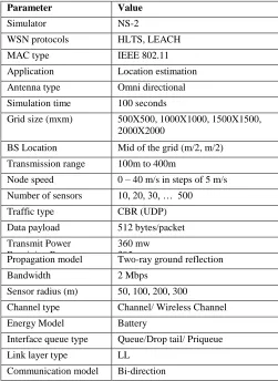
A traffic generator named cbrgen is developed to simulate constant bit rate (CBR) sources in NS-2. Each CBR packet size is 512 bytes . We have chosen two-ray ground reflection model. MAC layer uses IEEE 802.11 DCF (distributed coordination function). A mobility generator named setdest is developed to simulate node movement. For fairness, identical mobility and traffic scenarios are used across protocols. Important simulation parameters are summarized in Table I.

Table I: Network configuration parameters

Parameter Value

Simulator NS-2

WSN protocols HLTS, LEACH

MAC type IEEE 802.11

Application Location estimation Antenna type Omni directional Simulation time 100 seconds

Grid size (mxm) 500X500, 1000X1000, 1500X1500, 2000X2000

BS Location Mid of the grid (m/2, m/2) Transmission range 100m to 400m

Node speed 0 – 40 m/s in steps of 5 m/s Number of sensors 10, 20, 30, … 500

Traffic type CBR (UDP)

Data payload 512 bytes/packet Transmit Power

Receiving Power Idle Power Initial Energy

360 mw 395 mw 335 mw 12 J

Propagation model Two-ray ground reflection

Bandwidth 2 Mbps

Sensor radius (m) 50, 100, 200, 300

Channel type Channel/ Wireless Channel Energy Model Battery

Interface queue type Queue/Drop tail/ Priqueue Link layer type LL

5. RESULTS AND DISCUSSION

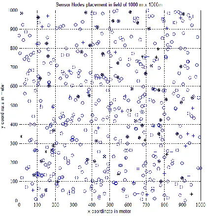
Figure 2 shows the initial field distribution of the network. A 1000m*1000m field is taken and nodes are randomly placed in it. The sink/base station (BS), which is denoted by x, is placed at the center of the field (500, 500). Placing the base station at the center is convenient so that no node founds it out of its transmission range. Here, the advanced nodes are shown by a plus symbol (+) and the normal nodes by a circle ( 0). In Figure 2, all the nodes are alive in the network.

The performance of our proposed HLTS is compared with the LEACH –Low Energy Adaptive Clustering Hierarchy protocol. We evaluated the following performance metrics:

Figure 2: Sensor nodes distribution in 1000m x 1000m field

Figure 3: Number of sensors vs. network lifetime

Network lifetime: The network lifetime is directly proportional to the number of live nodes in the network after during the simulation time.

Average energy consumption: The average energy consumed by the nodes in receiving and sending the packets.

Error ratio: number of time false target detected or mismatched.

Target detection probability: A fundamental challenge for these WSNs is to meet stringent QoS requirements including high target detection probability, low false alarm rate and bounded detection delay. It is measure the sensing performance of the network.

5.1 Based on Number of Sensors

When more sensors are deployed, each target is covered by more sensors, thus more set covers can be formed. Also considering the same number of sensors for a smaller number of targets the lifetime increases. The network lifetime increases with number of sensors and sensing range as shown in figure 3. The HLTS has 10-20% higher network lifetime as compared to LEACH even when sensing range is higher.

The network lifetime is directly proportional to the number of nodes in the network. Initially figure 4 show the increase in the network lifetime as number of nodes in the increase. But after 300 nodes (in 1000m x1000m) both protocols network lifetime (number of rounds) decreases. HLTS performs better in terms of number of rounds (i.e. measure in time).

In figure 5 the effect of network density on target detection and estimated the performance. When numbers of sensors are less the target detection probability is low but after increasing the sensor nodes up to 300 with transmission range of 100m the probability goes up to 90 to 95%. HLTS gives more accurate detection with less overhead as it involve limited number of nodes for detection i.e. parent and grandparent nodes. It reaches 98% accuracy with less mobility target when heavy networks.

40

Figure 5: Number of sensor nodes vs. Probability of target detection

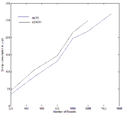
Figure 6: Number of rounds vs. total network energy consumption

5.2 Energy Consumption

In the proposed algorithm HLTS the energy consumed is reduced since only activated nodes in the network is involved in network and rest of nodes remain in standby mode. Figure 6 show the graph comparing the energy consumption between LEACH and HLTS.

5.3 Based on Transmission Range

When a target detected as it entered into the radio range of a sensor, the sensor output become 0 immediately after the detection and kept toggling between 0 and 1 as target moved towards the sensor. This is aimed due to minimizing false alarms at the cost of some missed detection. When the target paths are smooth enough our proposed algorithm HLTS gives excellent performance in terms of identifying and tracking different target trajectories as compared to LEACH as shown in figure 7.

Figure 7: Transmission range vs. Probability of target detection

Figure 8: Target speed vs. Error Ratio

5.4 Error Ratio

Error ratios are measure against the target speed in figure 8. As the target speed increases the error ratio also increases for both the algorithms. When target are less mobile the error ratio i.e. target not detected or wrongly detected or misplaced is 5% but when speed of target is 50 km/hour the error ratio increase to 30%. HLTS provide steady results over the speed.

6. CONCLUSIONS

7. ACKNOWLEDGMENTS

We thank anonymous referees for their valuable comments which helped in improving the content and presentation of the paper. We thank vice chancellor and director SOCIS of Indira Gandhi National Open University, New Delhi for always encouraging for the best.

8. REFERENCES

[1] I.F. Akyildiz, W. Su, Y. Sankarasubramaniam, E. Cayirci “A Survey on sensor networks ” IEEE Communication Magazine, pp. 393–422, 2002.

[2] Kemal Akkaya, Mohamed Younis “A survey on routing protocols for wireless sensor networks” IEEE Communication Magazine on Ad Hoc Networks , pp. 325– 349, 2005.

[3] Ameer Ahmed Abbasi, Mohamed Younis “A survey on clustering algorithms for wireless sensor networks”IEEE Communication Magazine, pp. 2826–2841, 2007.

[4] Wendi Rabiner Heinzelman, Anantha Ch, and Hari Balakrishnan. Energy-efficient communication protocol for wireless microsensor networks. pages 3005- 3014, 2000. [5] M. Bern R. Dahab L. B. Oliveira, H. C. Wong and A. A. F.

Loureiro. Secleach - a random key distribution solution for securing clustered sensor networks. In Fifth IEEE International Symposium on Network Computing and Applications, pages 145-154, Washington, DC, USA, 2006. [6] L. B. Oliveira E. Habib H. C. Wong A. C. Ferreira, M. A.

Vilaa and A. A. Loureiro “Security of cluster-based communication protocols for wireless sensor networks.” In 4th IEEE International Conference on Networking (ICN05),

volume Lecture Notes in Computer Science, pages 449-458, Washington, DC, USA, 2005.

[7] Washington, DC, USA, 2007. A. V. Reddy R. Srinath and R. Srinivasan. Ac: Cluster based secure routing protocol for wsn. In Third International Conference on Networking and Services, page 45, Washington, DC, USA, 2007.

[8] Y. Geng C. Hong-bing and H. Su-jun. Nhrpa: a novel hierarchical routing protocol algorithm for wireless sensor networks. China Universities of Posts and Telecommunications, September 2008.

[9] M. A. Vilaa H. C. Wong M. Bern R. Dahab L. B. Oliveira, A. Ferreira and A. A. F. Loureiro. Secleach-on the security of clustered sensor networks. (87(12)):2882-2895, December 2007.

[10]G. Hu D. Wu and G. Ni. Research and improve on secure routing protocols in wireless sensor networks. In 4th IEEE International Conference on Circuits and Systems for Communications (ICCSC 2008).

[11]C.Wang K. Zhang and C.Wang. A secure routing protocol for cluster-based wireless sensor networks using group key management. In 4th IEEE International conference on Wireless Communications, Networking and Mobile Computing (WiCOM08).