Regime Shift in Antitrust

Munich Personal RePEc Archive

Regime Shift in Antitrust

Ghosal, Vivek

February 2007

Online at

https://mpra.ub.uni-muenchen.de/5460/

Regime Shift in Antitrust

Vivek Ghosal*

February 2007

Abstract

This paper empirically models the longer-run deep-seated shift in intellectual thinking that followed the Chicago School’s criticism of the older antitrust doctrine, the shorter-run driving forces related to switches of the political party in power, merger waves, changes in economic activity and the level of funding and quantifies their impact on enforcement by the Antitrust Division of the U.S. Department

of Justice over the period 1958-2002. The key findings are: (1) a distinct regime-shift in antitrust

enforcement during the 1970s and, post-regime-shift, there has been a marked compositional change with a quantitatively large increase (decrease) in criminal (civil) antitrust court cases initiated; (2) post-regime-shift, there appears to be a change in the role played by politics with Republicans initiating more (less) criminal (civil) court cases than Democrats and the estimated quantitative effects are large; (3) disaggregating the total number of court cases into the main categories under which they are initiated (price-fixing, mergers, monopolization and restraints-of-trade) shows that individual types of cases have widely differing responses to changes in the driving forces; and (4) in a horse-race between the regime-shift and political effect on one side and the remaining variables on the other, the former forces win hands-down in explaining broad shifts in enforcement. Modeling the longer-run shift and disaggregating the court cases emerge as crucial to gaining insights into the intertemporal shifts in enforcement. The paper elaborates on the causes for the shift in enforcement and on the effectiveness of antitrust.

Keywords: Antitrust enforcement; regime-shift; politics; supreme court; effectiveness.

JEL: L40; K00.

* School of Economics, Georgia Institute of Technology, Atlanta, GA 30332; CESifo (Munich); and

ENCORE (Amsterdam). Contact: http://www.econ.gatech.edu/faculty/vivek-ghosal/

1. Introduction

Dating back to 1890, when the first major antitrust law was enacted in the form of the Sherman Act,

the U.S. has perhaps had the richest history of antitrust enforcement with a complex confluence of

economic, legal and political forces producing ebb and flow in enforcement.1 As described in

Harrington (2006): “Antitrust enforcement is the process by which a more competitive environment is

created through the prohibition of certain practices deemed illegal by antitrust laws.” More broadly,

the objectives of antitrust can be thought of as fostering competitive markets and promoting

innovation, with implications for prices, welfare and economic growth. While historically the US has

had active enforcement,2 the recent past has seen competition policy gaining emphasis in other parts

of the world. The European Union has seen important changes in the enforcement of collusion and

mergers, and calls for greater vigilance to ensure competitiveness.3 Japan and Australia have put new

emphasis on competition policy and debated harmonizing laws with major trading partners (Cassidy

(2001), Homma (2002), OECD (1999) and Richardson and Graham (1997)). Against the backdrop of

the historical US perspective, the changing global emphasis and the potential role played by

competition policy in shaping the competitive dynamism of economies, the primary objective of this

paper is to examine how changes in intellectual thinking, shifts in the legal landscape and political

forces have influenced the intertemporal path of antitrust enforcement by the Antitrust Division of

1

In spite of it being in large part a political response to undesirable business conduct and emergence of large corporations, scholars have noted the close match of the wording of Sherman Act section 1 (restraints of trade) and section 2 (monopolization) to those of Adam Smith on collusion and monopoly power (Blair and Kaserman, 1985). See Bork (1966) and Lande (1982) for debates on the intent of the Sherman Act. Motta (2004, 1-9) provides a succinct history of the U.S. antitrust enforcement.

2

Oz Shy (1995, p.5) writes: “.in the US real prices of products tend to be the lowest in the world. The US also has the most restrictive antitrust regulation structure in the world. Hence, although it is commonly argued that market intervention in the form of regulation results in higher consumer prices, here we observe that antitrust regulation is probably the cause for low consumer prices in the US...”

3

Contributions in Eekhoff (2004) make a case for competition policy vigilance in the newly deregulated sectors in Europe to ensure competition and growth. Enforcement of cartels in Europe has seen a big change; Harding and Joshua (2004) detail the shifts. Duso, Neven and Röller (2003) and Bergman,

Jakobsson and Razo (2003) present analysis of EU merger enforcement. Motta (2004, p.9-17) provides

the U.S. Department of Justice.4 Below we discuss these driving forces.

We begin by focusing on the more deep-seated changes that occur relatively infrequently.

The influence of the Chicago School is well documented and the genesis of their law and economics

movement is often recognized to be Aaron Director and Edward Levi.5 Director and Levi (1956)

criticized the state of antitrust, disagreed with a variety of business practices like tying and vertical

restrictions being anti-competitive and abuse of monopoly power, downplayed the likelihood of

predatory pricing, emphasized efficiencies and noted flaws in key antitrust decisions like Standard

Oil (1911) and Alcoa (1947).6 In similar tone, Director (1957) criticized the United Shoe Machinery

(1968) decision. Many of these arguments went on to become guideposts for the Chicago School’s

law and economics thrust. The influential contributions by Stigler (1964) and Williamson (1968),

along with Demsetz (1973, 1974), Bork (1966, 1978)7 and Posner (1969, 1974, 1976) among others,

solidified the law and economics framework. The shift in thinking was as follows. First, vertical and

conglomerate mergers, resale price maintenance, vertical restrictions and other conduct that were

often viewed as anti-competitive under the older antitrust regime were given pro-competitive and

efficiency interpretations. Second, the focus shifted to areas of clearer harm to welfare such as

price-fixing and horizontal mergers in concentrated markets. Baker (2002, 2003), Crandall and Winston

(2003), Kovacic and Shapiro (2000) and Motta (2004, p.2-9) provide discussion of these shifts.

4

The U.S. enforcement is conducted by the Antitrust Division of the Department of Justice and the Federal Trade Commission. The Antitrust Division is solely responsible for criminal prosecutions. Merger control in contrast is shared by the two agencies. In this paper we only focus on the Antitrust Division in part because it represents the totality of criminal enforcement and in part because disaggregated data on enforcement under the various Antitrust Acts were available for the Division.

5

Director joined the Chicago Law faculty in 1946, founded the Journal of Law and Economics in 1958, and his students included Robert Bork, Frank Easterbrook and Richard Posner – legal scholars and judges who greatly influenced antitrust. Bork notes: “[Director’s] teachings...made him the seminal figure in launching the law and economics movement, which transformed wide areas of legal scholarship.” (From: Aaron Director, Founder of the Field of Law and Economics, University of Chicago Press, 2004.)

6 _{Influenced by Director’s hypothesis that firms would prefer mergers and other practices to attain} monopoly status as opposed to predatory pricing, McGee (1958) tested whether Standard Oil engaged in predatory pricing, a key issue in the 1911 antitrust decision. His results suggested this was not the case.

Given this new intellectual thinking, there is the likelihood of a regime-shift in antitrust enforcement.

While much has been written on this, there has been no formal attempt to empirically model this

longer-run shift and quantify the effects using antitrust enforcement data. In this paper we use

econometric techniques to detect potential regime-shift in enforcement and control for it when

examining the impact of the political and other shorter-run driving forces.

Turning to the legal arena, the US Supreme Court is the final arbitrator of antitrust court

cases. Pate (2004) presents an overview of the key role played by the Supreme Court in shaping US

antitrust. Firms being prosecuted can appeal to this highest court for relief. The Antitrust Division

can appeal to the Supreme Court if they lose in lower courts. The Court’s decisions become landmark

one’s and influence future enforcement. The Supreme Court justices are nominated by the President

and confirmed by the Senate. Republican Presidents are expected to appoint more conservative

justices. The Republican-nominated justices of the Court had a simple majority during 1958-62, were

in the minority during 1963-69, regained a simple majority during 1970-71 and attained a

commanding two-thirds majority starting 1972 which they have not relinquished. Given the shift to a

more conservative court and very likely a more laissez-faire perspective on economic activity, it is

plausible that the stance on antitrust may have shifted. We return to this discussion in section 8.

The political spectrum is the more time-varying element due to changes in the party in power.

The literature has thought about political attitudes towards regulation or interference in markets in

alternative ways: costs v. benefits of regulation; probability of bureaucrats making mistakes resulting

in different degrees of confidence in bureaucracy; income redistribution; and paternalistic views. For

our purposes we distinguish between a relatively conservative hands-off v. a more liberal hands-on

approach to markets. This categorization is common, see Bailey and Chang (2001) and the references

there. Over our sample period (1958-2002) there have been ten different Presidents and six switches

of the party in power, allowing us to measure the impact of political changes on enforcement.

Studying the linkage between politics and enforcement is interesting due to the Antitrust Division’s

General who heads the Antitrust Division: the relationship is akin to a Principal-Agent one and

analogous to the affiliated-regulator setting described in Faure-Grimaud and Martimort (2003). This

potentially sets the stage for shifts in enforcement with switches of the party in power.

Apart from the above, we focus on other broad shorter-run driving forces that may affect

enforcement such as merger waves in the economy, funding for the Antitrust Division and the level

of economic activity. As part of our additional results, we examine the role played by foreign

competition and the political composition of the U.S. House of Representatives and the Senate.

This paper contains several features that distinguish it from previous studies. First, prior

empirical studies did not model the run effects and certainly not jointly modeled the

longer-and-shorter run driving forces. Longer-run shifts could arise from deep-seated changes in intellectual

thinking about business conduct. As we demonstrate in sections 4 and 5, the antitrust enforcement

data show longer-run shift in their levels, symptomatic of structural-breaks. Shorter-run fluctuations

may arise from merger waves, shifts of the political party in power, economic conditions, the level of

funding available for investigations, among others. Our empirical results show that omitting the

control for the structural-break significantly reduces our understanding of the intertemporal path of

enforcement and generates erroneous inferences about the shorter-run effects. Second, in contrast to

the previous literature, we analyze antitrust data at several levels of disaggregation. The grand total

number of court cases filed are first disaggregated into total criminal and total civil cases as they

represent very different types of violations. Criminal court cases relate to price-fixing, bid-rigging

and market-allocation schemes; these are per se violations with no efficiency justification. In

contrast, civil court cases relate to mergers, exclusive contracts, tying agreements, bundling, vertical

restraints, among others, and have market power v. efficiency considerations and rule of reason

prevails where the specific business conduct is judged by the party’s intent and the effect the conduct

is likely to have. Next, we disaggregate the total civil cases into the three main components: Clayton

Act section 7 (mergers) and Sherman Act sections 1 (restraints of trade) and 2 (monopolization).

violations can be quite different, such as mergers and tying agreements. Our estimates show that the

longer-run and shorter-run driving forces often have divergent sign patterns and varying quantitative

effects on these different types of cases, vividly demonstrating that aggregation masks underlying

heterogeneity. Third, we control for the total number of mergers in the US as merger evaluation is

one of the primary tasks of the Antitrust Division, using up significant resources. This allows us to

control for the Division’s workload, examine the link between merger waves and enforcement, and

whether when merger investigations increase, is there reduction of enforcement in other categories.

Fourth, in section 6 we test for endogeneity of funding for the Antitrust Division and the US merger

wave to the prevailing enforcement stance: e.g., vigorous merger enforcement may dampen merging

spirits. Fifth, we study enforcement data over a long 45-year period, 1958-2002. These aspects make

this one of the most comprehensive econometric studies of US antitrust enforcement. Since the

abstract summarizes the key results, we do not repeat them here.

In section 2 we review some theoretical contributions, provide details about the institutional

setting of the Antitrust Division and summarize previous empirical findings. The empirical model,

econometric issues related to identifying regime-shift in antitrust enforcement, data and endogeneity

of some model variables are presented in sections 3, 4, 5 and 6. Estimation results appear in section 7

and the paper concludes with a discussion of results and final remarks in sections 8 and 9.

2. Theory and Prior Empirical Findings

2.1. Some Insights from Theory

We review two papers that provide insights for our empirical analysis. Faure-Grimaud and Martimort

(2003) link the institutional structure of the regulatory agency with policy implementation across

political principals. The political principal ‘P’ delegates the task to regulatory agent ‘R’ and one of

their results relates to the extent to which R can be captured by the firms it is entrusted with

regulating. R can be (1) independent, implying that R stays as P changes or (2) affiliated, implying

that all principals dislike giving up rents to firms. Let P1 be more concerned with rent extraction and

less by efficiency than P2; ψ1<ψ2. They (p.418) interpret the gap ψ1-ψ2 as the degree of polarization.

In general, the independent-regulator can span several political principals, is longer-lived and has

greater scope for capture by firms; here the principal can change without significant changes in

enforcement. In contrast, the affiliated-regulator is shorter-lived, has less scope for being captured by

firms and can be dismissed by the principal if there is deviation from the desired policy stance. The

Assistant Attorney General (AAG) who heads the Antitrust Division is appointed by the US

President; the relationship is akin to a Principal-Agent one and fits the affiliated-regulator setting.8

We assume that the AAG will implement the President’s desired policy stance as doing so may lead

to future benefits like political and other appointments; else there could be removal from office and

denial of future rewards. Over 1958-2002 there have been 10 different Presidents and 21 AAGs

(excluding interim AAGs), indicating variation in both the principal and the agent. We note two

aspects for our analysis: (1) with the Antitrust Division’s affiliated-regulator setting, we potentially

expect a distinction between Republicans and Democrats in the intensity of enforcement; and (2) we

could proxy the gap ψ1-ψ2 by the difference in the level of enforcement between Republicans and

Democrats. In our empirical analysis, we estimate this gap and whether this has changed over time.

Second, Peltzman’s (1976) vote-maximizing regulator faces a trade-off between producer and

consumer interests. The group interests are captured by commodity price ‘p’ for consumers and

profits ‘π’ for producers. The regulator's objective function is M=M(p, π), with Mp<0, Mpp<0, Mπ>0,

Mππ<0 and Mpπ=0; the negative second-order conditions imply diminishing political returns to higher

π or lower p. The constraint is given by π=f(p, c), where c=production costs and c=c(q) with

q=output. This yields an equilibrium condition -(Mp/fp)=Mπ=-λ which states that the marginal

political product of a dollar of profits equals the marginal political product of a price cut that also

costs a dollar of profits. Thus, equilibrium will not result in protection for only one group. We focus

on two aspects for our empirical analysis: (1) re-write the regulator’s (specific) objection function as

M=log[πκ(A-p)φ], or M=κlogπ+φlog(A-p), where κ and φ are the weights attached to the relevant

group’s interests and A an arbitrary constant with A>p, satisfying the optimality conditions in

Peltzman’s model. Change in political regime could be conceptualized by change in κ and φ, with κ

higher under Republicans who we assume are more pro-business (or laissez faire) with less vigorous

enforcement; and (2) Peltzman’s (p. 225-227) results show that given the positive marginal consumer

(producer) opposition to higher (lower) prices (profits), the regulator will not force the entire

adjustment onto one group. Thus, in depressed profits during weak economic conditions, the political

wealth effect implies that the regulator’s incentive to let prices fall will be attenuated so prices would

not fall as far as they would in an unregulated setting; consumers will buffer some of the producer

losses. Thus antitrust enforcement will be relatively slack (vigorous) when economic conditions are

weaker (stronger), suggesting a direct relationship between economic conditions and enforcement.

2.2. Prior Empirical Findings

Several studies have analyzed the total number of antitrust court cases as they represent the

most visible action in enforcement; Ghosal and Gallo (2001) and Harrington (2006) briefly review

these studies. Using the Antitrust Division data, Posner (1970) did not find a relationship between the

party of the President and enforcement and he noted that enforcement appeared procyclical.

Lewis-Beck (1979) did not find evidence of Republicans, as measured by the Party of the President and the

composition of the House and Senate, pursuing less vigorous enforcement over 1890-1974; he found

that neither GDP growth nor unemployment rate explained variations in the number of cases

initiated. Siegfried (1975) found that economic factors do not influence enforcement. Cartwright and

Kamerschen (1985) did not find significant effect of the party of the President on the number of

cases. Pittman (1992) did not find evidence that political factors systematically affected antitrust

enforcement. Results in Ghosal and Gallo (2001) showed no effect of the party of the President, and

Tollison (1982) examined the link between political influence and case-activity and found support for

the private-interest theory of FTC behavior. Amacher, Higgins and Tollison (1985) found weak

evidence that Democratic dominated commissions pursued enforcement more vigorously; they found

no consistent link between economic activity and cases initiated. Coate, Higgins and McChesney

(1990) found some evidence in support of the interest-group hypotheses. Collectively, previous

empirical studies show that: (1) there is little systematic evidence that the party of the President

matters for antitrust enforcement; and (2) the relationship between economic activity and

case-activity is ambiguous – the typical finding being a weak positive, or no, link.

3. Empirical Specification

The behavior of economic agents often involves gradual adjustment of the relevant decision variable

to the desired (or equilibrium) levels. One modeling strategy is to consider a decision-maker’s

objective to minimize the expected present value of a quadratic loss function subject to adjustment

and disequilibrium costs. Since the theoretical and empirical underpinnings of this framework are

laid out in Gould (1968), Kennan (1979) and Treadway (1971), we do not repeat them here. We

assume that the Antitrust Division pursues court case activity subject to minimizing these two costs:

(1) adjustment costs arise for the Division due to resource constraints given by the number of

attorneys, economists and funding, implying that actual change in the Division’s case activity may be

less than the desired change in order to minimize adjustment costs; and (2) disequilibrium costs arise

as the Division is subject to pressures from the political arena and producer and consumer groups. If

the Division’s enforcement stance is above or below the desired level, there may be pressure to

rectify this, bringing the Division unwanted scrutiny and publicity.9 Thus the above framework may

be a useful way of modeling the intertemporal path of antitrust enforcement.10

We begin by defining our main variables: CASES=number of antitrust cases filed in court;

VIOL=number of (typically unobserved) violations; PRES=political party with PRES=1 if

Republican, else 0; REG=regime with REG=1 if new regime, else 0; FUND=funding allocated to the

antitrust division; WAVE=total number of mergers in the US; and ECON=economic conditions.

Formally, the Antitrust Division is expected to minimize the quadratic loss function:

], ) CASES CASES ( ) CASES CASES ( [ E CASES Min (1) 0 t 2 1 t t A 2 * t t D t t

∑

φ

φ

ρ

where CASESt is the actual number of court cases in year t, CASESt* is the desired number, φD and

φA are the disequilibrium and adjustment cost parameters and ρ is the constant discount factor. The

Antitrust Division makes a sequence of actual CASESt decisions designed to meet the target

CASESt* which is a function of relevant driving variables (described below). Since the derivations

are well documented in Gould (1968), Kennan (1979) and Treadway (1971), we don’t repeat them

here. Solving the model results in the partial-adjustment equation: CASESt-CASESt-1=λ(CASESt*

-CASESt-1), where the actual change in CASES is a fraction λ (0#λ#1) of the desired change, with λ

being a function of the adjustment and disequilibrium costs noted above. Rewrite the above as:

. CASES ) 1 ( CASES CASES

(2) _t =

λ

λ

The desired CASESt* is modeled as a function of the relevant driving variables. Below we

first outline our benchmark empirical specification and then address additional issues related to the

dynamics and lagged structure of the model variables. Let CASESt* be modeled as:

. υ ECON a

FUND a

WAVE a

REG a PRES a

VIOL a CASES

(3) _t* = _{1 t−1} + _{2 t−1} + _{3 t−1}+ _{4 t−1}+ _{5 t−1} + _{6 t−1} + _t

Since the relevant factors take time to impact the number of court cases, we use lagged values.11

CASESt* is driven by the number of (typically unobserved) violations, VIOL, assuming that it takes

time for information about possible violations to flow into the Antitrust Division; a1 is expected to be

positive. The Division’s willingness to initiate new cases in part depends on the prevailing political

stance, PRES, and regime, REG. A relatively hands-off markets stance may lead to fewer cases; a2

and a3 are expected to be negative. The US merger wave, WAVE, embeds multiple effects: (a)

increase in WAVE may imply an absolute increase in the number of mergers blocked, leading to an

increase in cases; (b) with an increase in WAVE, resources may have to be diverted to evaluate them,

taking resources away from other types of investigations; and (c) information discovered during

merger evaluation may unearth other violations, leading to increased cases.12 Thus, the sign of a4 is

ambiguous. The ability to initiate new cases depends in part on the level of funding, FUND. Since

current court cases typically result from past investigations, we use past funding as the relevant

variable which allows the Division to conduct investigations; a5 is expected to be positive.13 The

11

E.g., with a new political party in power, change in enforcement is not likely to be instantaneous. Also, potential violators get to observe the new regime and alter decisions with a lag. Merger and Sherman Act sections 1 and 2 investigations can be drawn out with information gathering, preliminary investigation and possible issuance of Civil Investigative Demands. The legislative process for funding starts two-years before the fiscal year in which they are needed and goes through various committees and subcommittees in the House and Senate, the Department of Justice and Office of Management and Budget.

12 _{E.g., while evaluating the pending merger between First Data Inc. and Concord EFS Inc. the Antitrust} Division discovered evidence on exclusivity contracts between Western Union and retail outlets, leading the Division to start an investigation of Western Union and issue Civil Investigative Demands. When investigating the UPM Kymmene-Bemis MACtac merger, price-fixing violations were uncovered.

13 _{The link between the Antitrust Division’s funding and cases and investigations may be a weak one due} to variation in utilization of economists and attorneys. During peak work-periods an economist or attorney can be simultaneously working on multiple investigations; this falls in off-peak periods. The staff

economic activity variable, ECON, is motivated by the results in Peltzman (1976) which suggests a

positive relationship. We assume the error term is iid: ut−(0,σu2).

Next we model the (typically unobserved) violations as:

. e CASES b

ECON b

WAVE b

REG b PRES b v VIOL

(4) _t = ₀ + _{1 t−1} + _{2 t−1} + _{3 t−1}+ _{4 t−1} + _{5 t−1}+ _t

In our empirical analysis we examine the total number of court cases filed as well as disaggregated

by specific types of violations. For example, price-fixing conspiracies take place in smoke-filled

rooms and are unobserved till information becomes available to the Antitrust Division. In the case of

mergers, the economy often goes through thousands of mergers per year and the number of mergers

that have serious market power implications are not ascertained without investigation. Similarly,

other violations such as restrictive trade practices and abuse of monopoly power are typically

unobserved till information becomes available. The way we visualize equation (4) is that there are

some driving forces that may cause violations to increase or decrease and we spell these out. We

assume that every period has some given number of (unobserved) violations v0. Regarding the factors

that influence the intertemporal variation in VIOL, we assume that these effects take time and use

lagged values. The presence of a conservative political party, PRES=1, and regime, REG=1, may

imply greater VIOL as firms may feel they can escape close scrutiny; b1 and b2 are expected to be

positive. During higher WAVE, firms may have an incentive to merge beyond the potential higher

profits motivation because the Division’s resources may be limited and thus the chances of escaping

an investigation may be higher. Overall, potential violators may be more inclined to engage in

anti-competitive behavior with the view that the Division is pre-occupied with evaluating mergers; b3>0.

The economic activity variable, ECON, controls for the potential link between economic conditions

and antitrust violations. In general, the direction of the relationship (sign of b5) is ambiguous. For

example, a large literature examines the formation of cartels and the stability of collusive agreements

(see Levenstein and Suslow, 2002). But the literature is not conclusive on whether this is more or less

likely during economic downturns. If the Antitrust Division is vigorously pursuing court cases,

CASES, then potential violations may be lower due to the greater likelihood of detection and

prosecution; b5<0. The error term is assumed to be iid: ut−(0,σe2).

Using equations (4), (3) and (2), we get:

, ε θFUND ] CASES ζ ECON γ WAVE δ REG β PRES [α c CASES (5) t 1 t 2 1 j j t j j t j j t j j t j j t j 0 t + + + + + + + = − = − − − − −

∑

where εt=(ut+a1et-1). Given the structure of equations (4), (3) and (2), apart from FUNDS which has

one-lag, all the other variables enter with two-lags. The coefficients in equation (5) are typically

combinations of the coefficients in equations (2), (3) and (4). Given our assumptions for ut and et,

and assuming zero covariance between ut and et, εt is a linear combination of two iid errors: εt−iid(0,

σu2+a12σe2). The error term εt is similar to a MA(1) process. Next, some additional comments

regarding the specification: (1) As noted earlier, we do not include current period variables in either

equations (3) or (4). This is because it is reasonable to assume that various effects take time (see

footnote 11); (2) In equation (5), the variables typically contain two annual lags. If we consider

deeper lags in equations (3) and (4), then equation (5) retains the same form but will include

additional lags and the error term εt could be higher-order MA(.) process. Our experiments showed

that deeper lags of the included variables were not significant. In section 7, we formally test for

higher-order MA(.) process; and (3) As noted in the introduction, two variables in equation (5) may

potentially be endogenous: the U.S. merger wave (WAVE) and the Antitrust Division’s funding

4. The Data

Our data are annual over 1958-2002. Data on disaggregated court cases were available starting 1958.

Data on antitrust court cases and funding are from the Antitrust Division workload statistics. Data on

the total number of mergers in the US are from the Federal Trade Commission merger series

(1958-1977) and Thompson’s Financials M&As (1978-2002). Data on the Republican v. Democratic

nominated Supreme Court justices are from the U.S. Supreme Court archives.

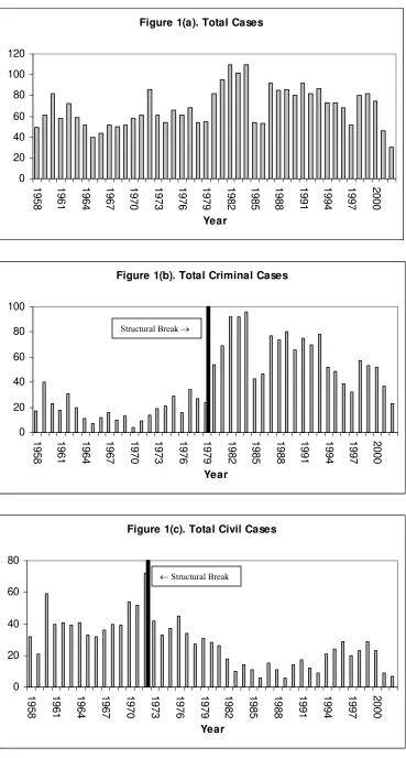
We examine antitrust enforcement data at different levels of disaggregation. A natural

pyramid is as follows. First is the total number of antitrust court cases filed in Figure 1(a); these data

show intertemporal fluctuations but no obvious trend. Second, the total cases are disaggregated into

the criminal and civil components in Figure 1(b) and Figure 1(c). The criminal component includes

per se violations such as price-fixing. The civil component includes mergers, monopolization and

restraints of trade cases. Our motivation for disaggregating the total cases was outlined in the

introduction. The data in figures 1(b) and 1(c) reveal longer-run drifts with criminal cases showing a

marked increase around the late-1970s and early-1980s and civil cases showing a decline after the

mid-1970s. In the latter part of the sample, the enforcement data reveal a stark compositional shift

with a greater proportion of criminal cases. We return to this issue when we discuss our empirical

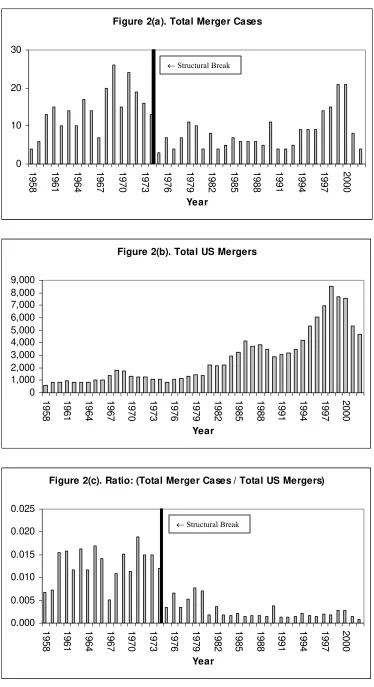
results in section 8. Third, the total civil cases are next disaggregated into the main Acts via which

they operate: Clayton Act section 7 (merger), Sherman Act section 1 (restraints of trade) and

Sherman Act section 2 (monopolization). Apart from data on the absolute number of merger court

cases filed in Figure 2(a), we also look at the ratio of merger court cases filed to the total number of

mergers in the US in Figure 2(c). Examining the ratio is meaningful as a merger wave in the US may

naturally result in an absolute increase in the number of mergers challenged. To get an idea of, for

example, whether the intensity of merger enforcement varies across political regimes, it is important

to deflate the total number of mergers challenged by the total number of mergers in the US. The

absolute number of mergers (figure 2a) show a decline in the early-1970s, remain low through the

cases filed to the total US mergers (figure 2c) shows a sharp decline around the mid-1970s with no

meaningful subsequent increase. Figures 3(a) and 3(b) plot the Sherman 1 and Sherman 2 cases

filed; the former shows a decline starting early 1980s and the latter sometime in the 1970s. Even a

cursory look at Figures 1-3 show significant differences in the intertemporal path of the different

types of cases, highlighting the perils of aggregation. Further, the data reveal distinct shifts in levels,

indicative of structural-breaks. Figure 4 displays the Antitrust Division’s real (deflated by the GDP

deflator) dollar funding. The level of funding generally increases till the late-1970s, declines over the

next decade before increasing starting the late-1980s. Funding (figure 4) declines during the very

period when criminal prosecutions increase (figure 1b), whereas the civil cases (figure 1c) and

funding show similar movements during the late-1970s and through the 1980s. Finally, we present

the political variables. Figure 5(a) displays data on the party of the President. Over our sample

period the US has had Republican Presidents for 24 years and Democrat for 20 years. In ancillary

specifications we include the Republican v. Democrat composition of the House and the Senate due

to their potential influence on the funding and other decisions.14 The data in Figure 5(b) show that

Republicans have had majority in the Senate for 13 years and in the House for only 8 years.

5. Detecting Regime Shift

In the introduction we discussed the potential reasons for expecting a regime-shift in enforcement

and several of the antitrust court case variables in section 4 revealed discernable shift in their levels,

indicative of structural-breaks. The precise break-date is unknown and we do not have an a priori

dummy variable to separate the before and after periods. The literature shows that if the data contain

a break-point and this is not known a priori, conventional hypothesis testing is not valid (Banerjee,

Lumsdaine and Stock, 1992). Given this, we use econometric techniques on detecting

break at an unknown date; Andrews (1993), Hamilton (1994, Ch.22), Stock (1994) and Stock and

Watson (1996, 2003) detail this methodology. Let τ the hypothesized break-date for the data on

CASESt. The dummy variable D(τ) is defined as Dt(τ)=0 for t#τ and Dt(τ)=1 for t>τ. An

autoregressive specification with an unknown break point τ is given by (H0: β=0):

. ) ( D CASES

c CASES )

6

( _{t t}

n

1 k

k t k

0

t = +

∑

ζ

β

τ

ω

= −

It is useful to clarify what an identified structural-break date means. Let data on CASESt be over

t=0,...,T and the statistical tests reveal a break-date in the year τ. In principle, nothing may have

changed in the year τ itself, but the sequence of events over t=τ+1,...,T result in a sample mean for

CASES that is different from t=0,...,τ. Regarding estimation, since the break-date is unknown, we

consider a series of dates between two potential dates τ0 and τ1. For each possible break-date, we

estimate equation (6) and get a F-statistic from testing H0: β=0. Since we test between τ0 and τ1, we

get a sequence of F-statistics and use the Quandt Likelihood Ratio (QLR) statistic to detect the break

point. The distribution of the QLR statistic depends on (1) the number of restrictions being tested q

(q=1 in equation 6) and (2) the width of the end-points τ0/T and τ1/T, where T is the total sample size

(Stock and Watson, 1996). For large sample approximations to the distribution of the QLR statistic to

be a good one, τ0 and τ1 cannot be too close to the sample endpoints. We follow Stock and Watson

(1996) and consider 15% trimming; i.e., τ0=0.15T and τ1=0.85T. Given our sample period of

1958-2002, this implies that we test for a potential structural-break over the window 1965 to 1996.15

Next we augment equation (6) to include additional explanatory variables as omission of

relevant variables may falsely generate a structural-break observation. The general form is given by:

, ) ( D ) ( D CASES c CASES ) 7

( _{t t t}

n 1 k k t k 0

t = +

∑

ζ

β

τ

τ

υ

= −

t t Φ'X

X Ψ'

where X is a vector of explanatory variables and Ψ and Φ the coefficient vectors. Using equation (7),

the null hypothesis is β=Φ=0. From equation (5), the components of X are PRES, FUND, WAVE

and ECON. The regime-shift variable REG is replaced by D(τ). For the interaction term, we only

consider one: D(τ)PRESt-1, the interaction between the regime-shift and the Presidential variable. Our

motivation, in part following our discussion of Faure-Grimaud and Martimort (2003), is to examine

possible changes in the enforcement gap over time between Republicans and Democrats. Finally,

some econometric issues: (1) for PRES, since the current and lagged values are identical for many

years, we only enter one-lag PRESt-1; and (2) several variables appear non-stationary – funding (fig.

4), total number of mergers (fig. 2b) and real GDP. We tested for non-stationarity using the

Augmented Dickey-Fuller and Phillips-Perron unit root tests (Enders, 1995, Ch.4). The tests could

not reject the null that the variables are difference stationary. Given this, we entered FUND, WAVE

and GDP in first-differences. The specification we estimate is:16

. FUND ] CASES ECON WAVE [ PRES ) ( D ) ( D PRES c CASES ) 8 ( t 1 t 2 1 j j t j j t j j t j 1 t t t 1 t 1 0 t

ε

θ

ζ

γ

δ

τ

ζ

τ

β

α

∑

We implemented the following sequence for estimation: (a) first we estimated equation (8).

Then we dropped all statistically insignificant second-lags. Insignificant first-lags were not dropped;

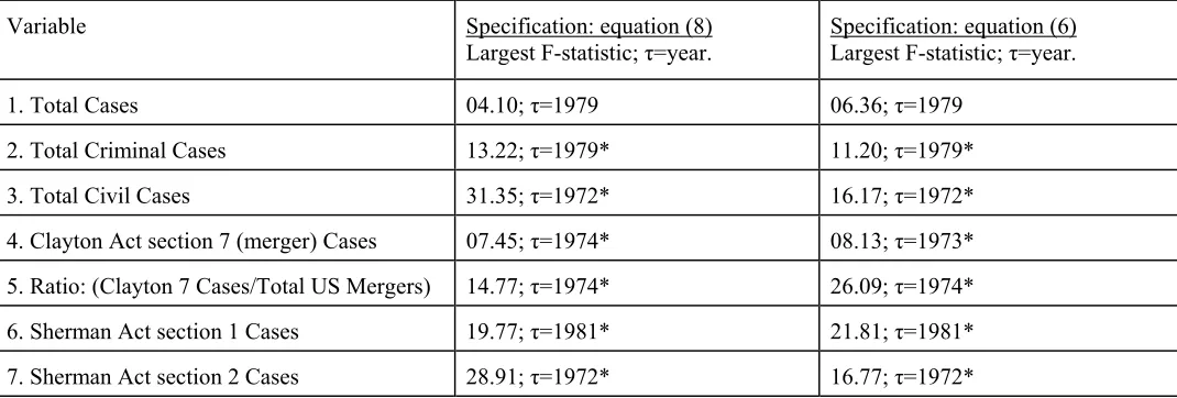
and (b) re-estimated equation (8) with the optimal lag lengths. We estimate both equations (6) and

(8) to detect structural-breaks. Table 1 summarizes the results for each type of case using D(τ)

ranging from 1965 to 1996. The estimated structural-break dates are basically the same across the

specifications. For the Clayton 7 (merger) cases, equation (8) reveals a break-date in 1974 whereas

equation (6) in 1973. Given the marginal difference and that (8) is a more complete specification, we

use 1974 as the break-date. The solid vertical black lines in figures 1(b), 1(c), 2(a), 2(c), 3(a) and 3(b)

show the estimated structural-break dates. In section 8, where we interpret and discuss our empirical

results, we comment on the implications of the estimated structural-break dates.

6. Potential Endogeneity

First, the Antitrust Division has to request funds, FUND, from the legislature. Requests for increase

in FUND may follow increase in CASES, potentially making FUND endogenous to CASES.

However, CASES is not the only factor influencing FUND; the complexity of cases, number of

internal investigations, party of the President, composition of the House and the Senate, among other

factors determine FUND. In addition, utilization of economists and attorneys (whose salaries are the

most significant component of the Antitrust Division’s annual budget) vary considerably over work

cycles. As noted in footnote 13, this variation in utilization poses a problem of clearly linking

investigations and CASES to FUNDS. Second, increase in CASES may dampen merging spirits,

potentially making the merger wave, WAVE, endogenous to CASES (merger challenges in

particular). Of course, CASES is not the only factor affecting WAVE. Shifts in technology, stock

market movements, deregulation, among other factors determine WAVE; see Jovanovic and

Rousseau (2001). Further, while only lagged values of FUND and WAVE enter equation (8), the

problem may be exacerbated as the error term is MA(.).

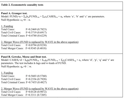
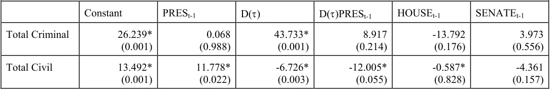
We use the Granger (1969) and Geweke, Meese and Dent (1983) procedures to test for

relationships between pairs of variables.17 Both test whether FUND and WAVE are exogenous (or

pre-determined) in a bivariate relationship with CASES. The Granger test examines whether

lagged-values of CASES affect current lagged-values of FUND and WAVE. The Geweke et al. test examines

whether lead-values of FUND and WAVE affect current CASES. Hamilton (1994, p.307-308)

provides a discussion of these tests. For FUND we conducted the following tests. For the Granger

test we regressed FUND on its own two lags and two lags of CASES: we regressed FUND on the

total number of cases as well as total civil and total criminal cases. For the Geweke et al. test, we

regressed CASES on two lags of FUND, two leads of FUND and two lags of CASES; as before, we

used data on total number of cases and total civil and total criminal. For the U.S. merger wave, we

replaced FUND with WAVE in the above equations. For WAVE, we report results for total civil

cases and total merger cases (Clayton 7) as these are the most relevant; criminal court cases are not

expected to be a factor in affecting U.S. merger waves. Table 2 presents the estimation details. Given

the F-statistics and significance levels, both FUND and WAVE are best treated as pre-determined. It

does not appear that, over our sample period, merger waves are endogenous to the Division’s merger

challenges. Factors such as technological change, stock market movements and deregulation are the

likely primary drivers of mergers. Neither is the Division’s level of funding jointly-determined with

the number of court cases, implying that case complexity, partisan politics, among others are the key

drivers. Given these results, we do not pursue instrumental variable estimation. OLS estimates

corrected for the MA(.) error structure will provide us with unbiased and consistent parameter

estimates and standard errors using the Newey-West (1987) procedure.

7. Estimation Results

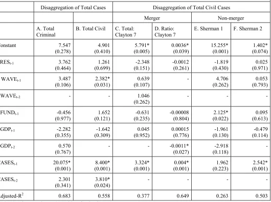
Table 4 presents the main results and several checks for robustness appear in Tables 5-7. The

interpretation of results and implications are postponed till section 8. In the estimated equation the

D(τ) dummies are replaced by the structural-break dates (table 1). As noted in section 5, only one-lag

of PRES is included and statistically insignificant second-lags of the other variables were dropped.

The error-structure is MA(1) (equation 5). To check whether a higher-order MA(.) representation is

needed – as would result from a richer lagged structure of equations (3) and (4) – we conducted

Lagrange-Multiplier tests. The test statistics in table 4 show that for total civil, Sherman 1 and

Sherman 2 cases we require MA(2), and MA(1) for total criminal, Clayton 7 and Ratio:Clayton 7.

Finally, except for the Constant, PRESt-1, D(τ) and D(τ)PRESt-1, the reported numbers are the

coefficient estimates multiplied by one-standard-deviation (one-s.d.) of the variable. Given the

considerable variation in the size of the estimated coefficients and means and standard deviations of

the variables, the estimates multiplied by one-s.d. gives us a ready look at the quantitative effect.

7.1. Main Results

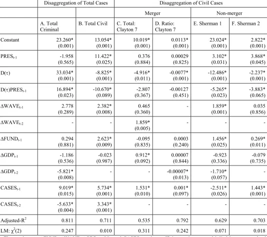
First we look at the results in Table 4 for total criminal cases (column A) and total civil cases

(column B). For the criminal cases prosecuted, the regime-shift dummy indicates a sharp increase in

the level from about 24 to 56 court cases per year. The PRES coefficient is insignificant indicating no

pre-regime-shift difference between Republicans and Democrats in their propensity to initiate

criminal cases. The D(τ)PRES interaction term, however, shows that post-regime shift the

Republicans, on average, have initiated about 17 more cases per year than Democrats. In terms of the

other variables, the merger wave has no impact on criminal cases. A one-s.d. decrease in real GDP,

with a lag of about two years, results in an increase of about 6 criminal cases. The estimate is highly

significant and the quantitative effect is economically meaningful: criminal cases prosecuted appear

to be countercyclical. Greater funding, has no effect on the number of criminal cases prosecuted.

Next we look at the estimates for the total civil cases initiated in column B. The regime-shift dummy

reveals a large drop in the level from about 13 to 4 cases per year. Similar to criminal cases, the

initiated about 11 more cases per year than Democrats. The D(τ)PRES interaction term, however, is

negative and large indicating that post-regime shift the Republicans have initiated about 10 fewer

civil cases per year. There appears to be a sharp reversal of the political effect before and after the

regime-shift. As we discuss below, the pre-regime-shift Republican effect is primarily being driven

by an increase in civil cases for about two years during the Nixon Presidency. In terms of the other

variables, total civil cases increase by about 2-3 following a one-s.d. increase in mergers in the US. A

similar result is obtained for the Division’s funding. Finally, there appears to be no significant

relationship between economic conditions and civil cases. A key point to note from columns A and B

is that, post-regime-shift, there is a clear compositional change in US antitrust enforcement: criminal

cases increase, civil cases decrease, and within the post-regime-shift period, Republicans initiate

more (less) criminal (civil) cases than the Democrats. We discuss this result in detail in section 8.

The total criminal cases and civil cases are next aggregated to get the grand total number of

court cases. Starting with Posner (1970), many studies have analyzed the total number of court cases

(see section 2). Since the total cases data do not show a structural-break (table 1), we do not include

the D(τ) and D(τ)PRES variables. Equation (9) – similar in specification to table 4, col. A and B –

presents the total cases regression (p-values are in parentheses).

38 . 0 R CASES 74 . 9 GDP 74 . 2 GDP 17 . 2 FUND 91 . 0 WAVE 64 . 5 PRES 23 . 8 02 . 34 CASES ) 9 ( 2 1 t ) 001 . 0 ( 2 t ) 182 . 0 ( 1 t ) 351 . 0 ( 1 t ) 554 . 0 ( 1 t ) 013 . 0 ( 1 t ) 112 . 0 ( ) 001 . 0 ( t = + Δ − Δ − Δ + Δ + + = − − − − − −

The PRES variable is positive and insignificant at conventional levels indicating that in the total

cases data we don’t find a clear political effect; this result is reminiscent of several previous studies.

Total cases increase following an increase in mergers in the US; this is similar to the result for total

civil cases (table 4, col. B). There is no meaningful relationship between funding and the total cases

initiated; this result is similar to the total criminal cases (table 4, col. A). And there is a weak

total civil cases (table 4, col. B). Finally, the adjusted-R2 is much lower than those in table 4. The

message from comparing the estimates in columns A and B of table 4 with the total cases results in

equation (9) above is that examining total cases data masks significant heterogeneity in the

underlying components, making inferences less meaningful.

Next we turn to the disaggregation of the total civil cases results presented in columns C

through F. For the total Clayton Act 7 (merger) court cases in column C, the regime-shift resulted in

a drop from about 10 to 5 cases per year. The PRES variable is insignificant and so is the D(τ)PRES

interaction term. These indicate no systematic political effect before or after the regime-shift in terms

of the merger cases filed. Similar results were obtained using the ratio (of merger cases filed to total

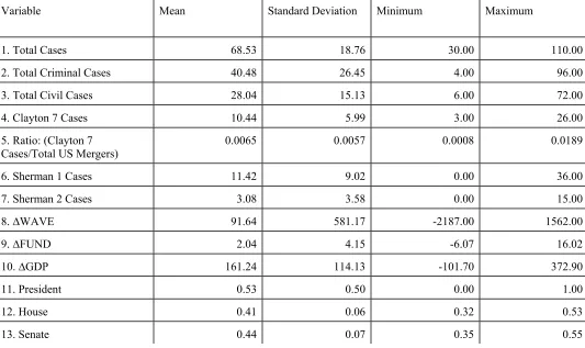
number of mergers in the US) variable (column D). The summary statistics in table 3 indicate that for

the sample period as a whole this ratio is 0.0065, implying that less than 1% of the mergers are

challenged. The regime-shift resulted in the intercept dropping from about 0.0113 to 0.0036, a large

quantitative effect. As in column C, the PRES and D(τ)PRES coefficients are insignificant in column

D. The Division’s funding appears to have no meaningful impact on the number of merger cases

filed. A one-s.d. increase in the number of mergers in the US, with a lag, results in about 2 additional

mergers challenged in court. While an increase in GDP appears to lead to an increase in the number

of mergers challenged (column C), the intensity of merger enforcement column D) falls with an

increase in GDP. In both columns C and D the quantitative effects are very small.

Finally we look at columns E and F, the Sherman Act section 1 (restraints of trade) and

Sherman Act section 2 (monopolization) court cases. The D(τ) estimates indicate a significantly

lower number of court cases post-regime-shift. For the Sherman 1 cases, the level drops from 23 to

11 cases per year and for Sherman Act 2 cases the drop is from 2.8 to 0.6 cases per year. These

represent large quantitative effects in terms of percentage declines. For both Sherman 1 and Sherman

2 cases, the signs on the PRES coefficient are positive indicating that the pre-regime-shift number of

cases were higher under Republican Presidents. And the signs on the D(τ)PRES interaction terms are

estimates imply a drop of 4-5 cases per year. The pre-regime-shift effect is similar to the total civil

cases results in column B. Pre-regime-shift, the Republicans were in power during the Nixon-Ford

administrations (1969-76), and we capture part (1958-60) of the Eisenhower administration. Our

examination of the data (figures 1c, 3a and 3b) indicate that the positive pre-regime-shift Republican

effect is being driven by outcomes from about two-years during the Nixon administration which saw

increases in Sherman Act (sections 1 and 2) cases; so this does not appear to be a pervasive

Republican effect, but a more idiosyncratic one from a couple of years of data. Overall, in terms of

the regime-shift and political effects, the total civil cases results in column B generally reflect the

patterns from columns E and F. In terms of the other variables, a one-s.d. increase in the Division’s

funding leads to an increase of about one case per year for Sherman 1 and even less for Sherman 2;

these are very small quantitative effects. The estimates of the WAVE coefficient show that a one-s.d.

increase in mergers in the US show an increase of about 2 Sherman 1 cases, and no impact on

Sherman 2 cases. Economic conditions, as measured by changes in GDP, have somewhat mixed and

relatively small quantitative effects on the Sherman 1 and 2 cases. The overall picture that emerges is

that changes in funding for the Antitrust Division, merger waves and fluctuations in economic

conditions appear to have rather small quantitative effects on antitrust court case activity. The

quantitative impacts are much larger for the regime-shift and Presidential effects.

Does Controlling for Regime-Shift Matter?

Table 5 presents results comparable to those in table 4, but without the regime-shift dummy

D(τ) and the D(τ)PRES interaction term. The results are quite different: the adjusted R2’s are lower;

not a single PRES coefficient is significant; only one GDP and one FUND coefficient is significant;

the WAVE coefficients display somewhat different significance patterns; and many of the lagged

CASES coefficients are larger – in part these may be picking up the effects of the omitted

regime-shift variable. Overall, controlling for regime-regime-shift appears quite important for detecting the influence

Does Disaggregation of Cases Matter?

First we disaggregated the grand total number of court cases into total criminal and total civil

(columns A and B in table 4). The differences are stark: the regime-shift effects have opposite signs

for criminal and civil cases; post-regime-shift, the political effect has opposite signs for criminal and

civil cases; change in GDP enters with opposite signs in the criminal and civil cases results; finding

is inconsequential for criminal cases but somewhat important for civil. Thus, it is not useful to lump

criminal and civil cases into one category – as many previous studies have done. Second, consider

the results in columns C through F. The estimated structural-break dates vary across the different

types of civil cases. For the regime-shift and political effects, the directional and qualitative effects

appear roughly similar for Sherman 1 and Sherman 2 cases but Clayton 7 merger cases follow a

different pattern – e.g., the Presidential effects are dramatically different. And funding, which matters

for the Sherman 1 and 2 cases, appears not important in merger cases. Thus it is not even useful to

lump the different types of civil cases into a total civil category. Overall, aggregation masks

heterogeneity and prevents us from getting a clearer look at the relationships.

7.2. Additional Results

Including House and Senate Effects

Appointments to the House and Senate judiciary committees depend on which political party

has majority and these may be important influences exerted on the Antitrust Division via the

budgetary and related processes. Also, the Assistant Attorney General has to brief the House and

Senate on its activities. To examine if this matters, we re-estimated the specification in table 4 after

including the percentage of Republicans in the House and in the Senate as additional controls. To

conserve space, in Table 6(a) we only present results for the total criminal and civil cases. The

House and Senate coefficients are all insignificant implying no meaningful effect. (While we do not

report these, the adjusted-R2s drop when we include these variables.) There are marginal differences

given that the House and Senate effects are insignificant it is not clear what this reduced significance

means. Overall, the inclusion of the House and Senate variables do not materially affect our broad

inferences on regime-shift, the party of the President or the other explanatory variables. This result

may not be terribly unexpected given that over our 45-year sample period, the Republicans have been

in the majority in the Senate for 13 years and in the House for only 8 years.

Including a Trend

One could argue that the merger cases data (figures 2a and 2c), for example, start high and

end up low, implying a negative trend. Similarly, the criminal cases (figure 1b) start low and end

high, implying a positive trend. Might controlling for a trend eliminate the regime-shift and political

effects we found in table 4? To investigate this, we re-estimated the specifications in table 4 by

adding a linear trend. To conserve space, in Table 6(b) we only report the total criminal and total

civil cases. The trend variable is (hopelessly) insignificant in both specifications. The results for the

total criminal cases remains intact. For total civil cases, the signs and the quantitative effects remain

intact but the significance levels of the D(τ) and D(τ) PRES coefficients drop. However, given the

very low significance levels of the trend coefficient – essentially implying a nuisance variable which

should be dropped form the regression – the crux of our inferences from table 4 remain intact.

Foreign Competition

Increase in foreign competition is likely to affect at least some areas of enforcement. Merger control

is an obvious one where the impact is expected via the product and geographic market definitions.

Foreign suppliers will provide competition in cases where products are relatively homogenous. Even

when products are differentiated, close substitutes may pose a competitive threat to domestic firms.

Ghosal (2002) provides an analysis of actual and potential foreign competition in antitrust. In short,

more foreign competition may expand the product and geographic markets reducing the likelihood

challenges by the Antitrust Division. For price-fixing, over the last 100 years the US has prosecuted a

large number of international and domestic cases. An increased number of firms in the market may

mean less ability to initiate and sustain collusive agreements. However, the Archer-Daniels Midlands

case showed that the entry of foreign suppliers in the market in part lead to the collusive agreement.

Thus, for price-fixing violations, the net effect seems uncertain. For restraints-of-trade (Sherman 1)

and monopolization (Sherman 2) categories it is not obvious whether increased foreign competition

is likely to increase or decrease such violations and the impact on the number of antitrust court cases

in these areas. Our only objective here is the check whether our main results from table 4 are affected

by including controls for foreign competition. The specific variable we considered is the ratio of US

merchandise imports to GDP (since services imports are a non-factor till the tail-end of our sample

period, we do not include this). The merchandise import-intensity averaged 3.05% during the 1960s,

6.06% during the 1970s, 8.35% during the 1980s, 9.61% during the 1990s, and just over 10%

thereafter. These numbers are not large and it is only in the 1990s does it get above the 10% mark.

We re-estimated equation (8) after including the import competition variable. Since our tests revealed

that the variable is clearly non-stationary in levels and stationary in first-differences, we entered it in

change form like GDP, WAVE and FUNDS. For total civil cases, Sherman 1 and Sherman 2 cases,

and the ratio of merger challenges to total US mergers, the import-intensity variable was

insignificant. For criminal cases, the second-lag is negative and significant and the quantitative effect

shows that a one-s.d. increase in ΔIMS leads to a decline of about 4 criminal cases with a two-year

lag. At face value, this suggests that more open markets with larger number of firms lead to less

price-fixing and less cases prosecuted. For total merger challenges, the first-lag is negative and

significant and implies that a one-s.d. increase in ΔIMS leads to one less merger challenge, a small

quantitative effect. Table 6(c) reports some of the results. The main point we note is that our central

Including Longer Lags

One could argue that including longer lags in equations (3) and (4) would result in a richer

specification in our estimating equation (8) and might capture instances where information flows

occur slowly and investigations are prolonged. To examine this we re-estimated the specifications in

table 4 with one additional lag; since our data are annual, this allows for a fairly deep lag structure

(including additional lags is tricky as it quickly erodes precious degrees of freedom). None of the

additional lags were significant. This is not surprising given that many of the second-lags in table 4

are insignificant. One exception was that the second-lag of ∆FUND appeared with a negative and

significant coefficient for criminal cases; but all other coefficients and inferences from table 4

remained intact. This negative coefficient at first glance is a bit puzzling. One likely explanation

might be that during the late-1970s and early-1980s when the number of criminal cases increased

considerably, the funding for the Antitrust Division dropped sharply (compare figure 1b with figure

4). Given that the other inferences did not change, we did not pursue this further.

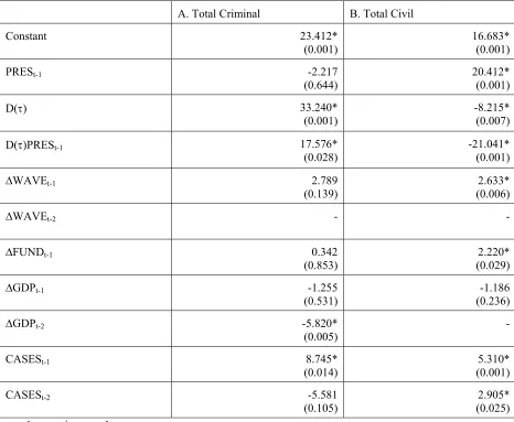
Joint Estimation of Total Criminal and Total Civil Cases

Our main results presented in table 4 were from single-equation estimation, implying that the

errors are uncorrelated across the different types of antitrust cases. Alternatively, one could think of

the problem as one of a “common manager” – the AAG for the Antitrust Division – for the different

types of cases and the decisions regarding one type of case are made in conjunction with the other

types. This interdependence could arise due to resource constraints (e.g., budget, attorneys and

economists) which may force substitution across cases (e.g., between criminal and civil). In this

scenario, the errors across the different types of cases may be correlated leading to potentially biased

inferences from the single-equation estimates in table 4. Since we do not have a structural model

from which we can get cross-equation restrictions to estimate a simultaneous equations system, we

instead estimated a Seemingly Unrelated Regressions (SUR) model which allows for error

columns A and B of table 4. The results in Table 7 show relatively minor differences in the

quantitative effects as compared to single-equation estimates presented in table 4; the qualitative

conclusions are the same. Our key inferences remain intact.

8. Discussion of Results

In this section we discuss our empirical findings. Since the regime-shift and political effects are our

main focus, we discuss these in greater detail and briefly comment on some of the other findings.

Regime-Shift

U.S. antitrust enforcement is a complex confluence of economic, legal and political forces

and significant shifts in enforcement will very likely have one or more of these factors as the key

drivers. We discuss these in turn for the civil and criminal cases and reiterate what we noted in

section 5 regarding the estimated structural-break date τ: in principle, nothing may change in the year

τ itself, but the sequence of events in the years t=τ+1,...,T result in a sample mean for antitrust court

cases that is different from the previous period t=0,...,τ.

For the civil cases (mergers, monopolization and restraints of trade), we noted the role played

by Stigler, Williamson, and others, in emphasizing the pro-competitive effects and efficiencies of

various types of business conduct. However, given the nature of US enforcement – e.g., to block a

merger, the Antitrust Division has to directly challenge the merger in court – unless the lawyers and

judges imbibe the new thinking, not much may change in terms of actual shifts in enforcement. That

the Chicago School legal scholars launched a powerful assault on the traditional antitrust mindset is

evident in the writings of Director, Bork, Posner, Landes, Easterbrook, among others. It is important

to note that historically the U.S. Supreme Court’s rulings have become landmark judgments (Pate,

to court and also act as a signal to firms as to what might be a legitimate challenge by the Division.18

A plausible premise is that a greater fraction of Republican-nominated conservative justices resulted

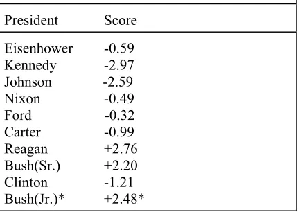
in a more laissez faire attitude towards economic activity.19 To examine changes in the Supreme

Court, we collected data on the justices: if they were appointed by a Republican President we

assigned a value of ‘1', else ‘0'. For a given year we tally up the scores and divide by nine (total for

Chief Justice and eight Associate Justices), giving us the fraction of Republican-nominated justices.

Figure 6 shows that the Supreme Court attained a commanding two-thirds Republican-nominated

majority in 1972 and have not lost it since then. Overall, one way to interpret the estimated

regime-shift dates for the civil cases is that they capture the turning points when the Chicago School’s law

and economics influences finally began turning the tide.

This, however, does not automatically explain why our estimated regime-shift dates vary

across different types of civil cases: 1974 for mergers, 1972 for Sherman 1 and 1981 for Sherman 2

cases. One plausible explanation may relate to the nature of specific cases that came up before the

court. We present two such cases that can arguably be identified as turning points:

(1) U.S. v. General Dynamics Co. (1974) where Justice Stewart delivered the opinion of the Supreme

Court that went against the antitrust mindset of the 1950s and 1960s and did not find a violation even

thought the existing market shares were high. The Antitrust Division had defined the product market

as “coal”. The Court disagreed with this definition and considered the market to be the more

18

E.g., courts have sided with the Antitrust Division that physicians cannot collectively bargain to set the fees they get from the insurers: Healthcare Partners Inc., 1995; Health Choice, St. Josephs Physicians Inc. and Heartland Health Systems, 1996. In equilibrium, physicians would have lower propensity to form such coalitions (at least explicit ones). In contrast, the Division lost several hospital merger cases: Mercy Health Services and Finley Tri-States Health Group, 1994; Long Island Jewish Medical Center, 1997. This may embolden hospitals to push more mergers. Legal precedence becomes an important factor.

19 _{Referring to the earlier enforcement, Bork (1978, p.4) wrote:}

“the Supreme Court, without compulsion by statute, and certainly without adequate explanation, has inhibited or destroyed a broad spectrum of useful business structures and practices.” Later (Bork, 1993, p.x-xi; reprint of the 1978 book) he wrote:

overarching “energy” which included oil, gas, nuclear and geothermal power. The Antitrust Division

had defined the geographic market narrowly. The Court disagreed with the geographic market

definition and broadened it considerably arguing that the market area should be defined in terms of

the transportation networks and freight charges that determine the cost of delivering coal and other

energy. In addition, the Court examined in detail the actual and potential competition and entry

conditions in the markets under consideration. This wide ranging evaluation of market conditions

was a radical departure from the narrow concentration based mindset of the earlier decades.20

(2) Continental TV v. GTE Sylvania (1977) where the Supreme Court emphasized concepts related to

competition in the market and argued that vertical restrictions are likely to promote interbrand

competition by allowing producers to achieve efficiencies in distribution. This is the first time that

the Court explicitly noted efficiencies to argue in favor of the pro-competitive effects.

These landmark cases roughly correspond to our estimated structural-break dates for the civil cases.

A more detailed examination of merger and other civil cases during this transition period along with

the specific rulings by the courts would shed greater light on the turning points for the specific types

of violations. Finally, some key administrative milestones for merger evaluation are (a) the

introduction of the Merger Guidelines in 1968 to streamline the procedures and (b) the 1976

Hart-Scott-Rodino act subsequent to which mergers above a certain valuation threshold had to be filed for

clearance. While our estimated 1974 structural-break date for mergers roughly falls in this window, it

seems that the shift in intellectual mindset about mergers and other business conduct and landmark

court decisions may be the more compelling forces explaining the regime-shift. It does not seem

persuasive that these administrative changes were, for example, more crucial than the landmark 1974

General Dynamics ruling by the Supreme Court.

For criminal cases, the explanation is potentially more complex. The estimated