MHD models for multi spacecraft / ground based data analysis and conjunction visualizations

Nikolai V. Pogorelov and Gary P. Zank

MHD Models for Multi-Spacecraft / Ground-based Data Analysis and Conjunction Visualizations

P. Daum and J.A. Wild

Department of Communication Systems, Lancaster University, InfoLab21, South Drive, Lancaster, LA1 4WA, United Kingdom

Abstract. The BATS-R-US MHD code is used to describe the large-scale

structure of the magnetosphere whereby the model parameters are constrained by multi spacecraft Cluster data in the post-noon high-latitude magnetopause region. We discuss the potentials of the model in combination with the ex-perimental data to accurately describe the dynamics of these regions in three-dimensions. A major aspect of this potential is to make predictions about the configuration of flux tubes at the magnetopause boundary and to visualize the open flux tubes passing by the spacecraft and observed simultaneously by iono-spheric radars.

1. Introduction

Today’s global computational models of the geospace environment provide large-scale detailed simulations. From the first global magnetohydrodynamic (MHD) simulation by Leboeuf et al. (1978), through the first three-dimensional MHD models (Brecht et al. 1982; Ogino 1986), to the codes in their present states the models have developed and can now be used to span the enormous distances present in the magnetosphere to fill the gaps between the point-to-point small-scale in situ measurements and the large-small-scale processes.

In this paper we present a comparison between magnetometer data from an outbound pass of the Cluster spacecraft through the post-noon high-latitude magnetopause region together with simultaneous ionospheric data obtained by the CUTLASS radars for 14 February 2001 (Wild et al. 2001), and a global MHD model simulation. The main focus lies on the processes at the magnetopause boundary layer. Here in particular we are interested in flux transfer events (FTE) as first described by Haerendel et al. (1978) and Russel & Elphic (1978). FTEs can be seen in the spacecraft data mainly as bipolar signatures in the field component normal to the magnetopause and in an enhanced total magnetic field strength. Pinnock et al. (1995) and Provan et al. (1998) described the ionospheric coherent radar signatures of FTEs as “pulsed ionospheric flows”, poleward-moving regions of enhanced convection flow in the dayside auroral zone. These are also often seen as poleward-moving regions of backscatter or enhanced backscatter power, the radar counterpart of “poleward-moving auroral forms” (PMAFs), are widely accepted to be the signature of FTEs (Sandholt et al. 1990; Thorolfsson et al. 2000). The measurements of the radar and the Cluster spacecraft represent a point-to-point signature of the FTEs, to quantify the process a global MHD simulation is performed in order to describe the three-dimensional dynamics between these two point measurements and to establish a

different approach than the predominant Cooling-Model method (Cooling et al. 2001), which is limited to be two-dimensional at the boundary.

2. Instrumentation

2.1. Radar data

The ground-based instruments employed in this study are the pair of CUTLASS radars. CUTLASS is an HF coherent backscatter radar system located at Han-kasalmi, Finland and _Þykkvibær, Iceland, and forms part of the SuperDARN array (Greenwald et al. 1995) together with the EISCAT Svalbard radars it is an essential ground-based diagnostic tool for the studies of the cusp/cleft region of the magnetosphere being carried out with the Cluster mission. A fully detailed description of the radar system employed in this study can be found in Wild et al. (2001).

2.2. Cluster FGM magnetometer data

The ESA Cluster mission allows for the first time the study of three-dimensional spatial and temporal characteristics of the geospace environment (Escoubet et al. 1997). The mission consists of four identical spacecrafts orbiting the Earth in a tetrahedral formation. Each Cluster spacecraft is equipped with an identical payload of particle and field instruments. In this study we concentrate on the fluxgate magnetometer (FGM) experiment (Balogh et al. 1997), which is pro-viding accurate, high time-resolution measurements of the magnetic field vector (up to 67 vectors/s). The principal period of interest for this study is_∼09:00– 11:00 UT, when Cluster were at a radial distance of _∼11–13 RE in the region

of the high-latitude magnetopause, because of the small spatial separation of the spacecraft compared to distances in the magnetosphere, we concentrate here just on the Cluster-1 (Rumba) spacecraft.

3. Observations of the Cluster spacecraft and the radars

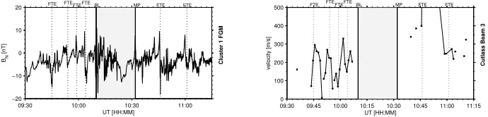
In the left panel of Fig. 1 we display the Cluster-1BN component of the boundary

normal coordinates (Russel & Elphic 1978), whereN is the estimated outward normal to the magnetopause, determined by the minimum variance method (Sonnerup & Cahill 1967). We note that magnetospheric FTEs are observed

∼09:45,∼09:54,∼09:59,∼10:04,∼10:46, and∼11:01 UT, indicated by bipolar maximum-to-minimum excursions in the BN component. The second panel in

09:30 10:00 10:30 11:00 −20

−10 0 10 20

BN

[nT]

UT [HH:MM]

FTE FTEFTEFTE BL MP FTE FTE

Cluster 1 FGM

09:300 09:45 10:00 10:15 10:30 10:45 11:00 11:15 100

200 300 400 500

velocity [m/s]

UT [HH:MM]

FTE FTEFTEFTE BL MP FTE FTE

Cutlass Beam 3

Figure 1. The first panel shows the magnetic field observation by the Cluster-1 spacecraft of the BN field component. The vertical dashed lines

represent the time of identified FTEs, BL the inner edge of the magnetopause boundary layer and MP the last magnetopause current sheet crossing. The second panel shows the time-series of the Doppler shift measurements from the lower-latitude backscatter region of the CUTLASS Finland beam 3, averaged over∼74.5◦–76◦ magnetic latitude.

4. MHD simulation

4.1. BATS-R-US MHD Model

The Block Adaptive-tree Solar-wind Roe-type Upwind Scheme (BATS-R-US) model, was developed by the Computational MHD Group at the University of Michigan (Gombosi et al. 2001; Powell et al. 1999). It is based on a block adap-tive cartesian grid with block based domain decomposition, and it employs the Message Passing Interface (MPI) standard for parallel execution. The BATS-R-US model involved in this study is Version 7.73 which incorporates the Rice Convection Model (RCM) (De Zeeuw et al. 2004). The BATS-R-US model and the RCM model are part of the Space Weather Modeling Framework (T´oth et al. 2005). Simulation results have been provided by the Community Coordi-nated Modeling Center at Goddard Space Flight Center. The simulation condi-tions were set to BATS-R-US and RCM, dipole orientation consistent with real time, time-dependent inflow boundary conditions obtained from ACE plasma and magnetic field Level 2 data and the simulation grid was set to 1,958,688 cells.

4.2. VisAn MHD

The simulation results obtained from the BATS-R-US were processed with the VisAn MHD toolbox for Matlab°r _{(Daum 2006). At the present state VisAn}

includes tools for the BATS-R-US, the OpenGGCM, the Ogino MHD code, and preparations for the Lyon–Fedder–Mobarry (LFM) code. It performs the necessary coordinate and data file transformations to convert the different raw model data to a Matlab°r _{conform standard. The toolbox also performs the}

necessary interpolations to create the monotonic 3D plaid matrices, which are needed for the 3D plots. The Toolbox is fully compatible with the Matlab°r

standards and can be invoked by pre-existing application.

4.3. Simulation

the plasma density obtained from ACE to 50% of the original value. Former runs show that the BATS-R-US model has an earlier positive signature in theBy

component than the Cluster data which indicates that the boundary is pushed to a lower radial position. By comparing the model data with the Sibeck et al. (1991) boundary and the measurements obtained from Cluster, it can be found that by decreasing the density the boundary layer coincident with the Clster observation at ∼10:08 UT (Daum & Wild 2006).

5. MHD result and real data comparison

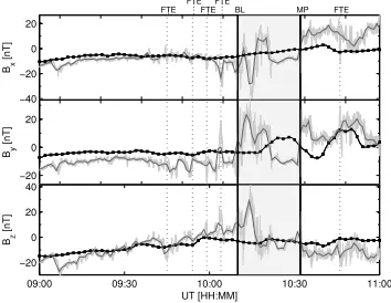
Figure 2 shows the comparison of the magnetic field data from the Cluster-1 spacecraft with the model output. The simulation results reproduce the general trend in the real data well, although the simulation does not reproduce major changes, which occur on a timescale of a few minutes or less, especially not the fast dips in the real data. The correlation coefficient is _∼70% for the averaged data without the grey shaded area. Inside the grey shaded area, from the inner magnetopause boundary layer to the last magnetopause crossing, the simulation cannot accurately describe the highly variable magnetic field.

−40 −20 0 20

Bx

[nT]

FTE: FTE:: FTE:FTE:: BL MP FTE:

−20 0 20

By

[nT]

09:00 09:30 10:00 10:30 11:00 −20

0 20 40

Bz

[nT]

UT [HH:MM]

Figure 2. The magnetic field vectors observed by the Cluster-1 spacecraft in a GSM frame. The solid dark grey line indicates the measurements averaged on an 1 minute interval, the solid black line with squares is the corresponding model output. The dashed lines are as in Fig. 1.

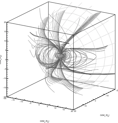
In order to get a first three-dimensional impression of the processes, the structure of the magnetic field configuration for 10:46 UT (FTE with dominant bipolar structure in theBN component) is shown in Fig. 3. It can be seen that

the magnetic field line configurations are similar to the ones first mentioned by Russel & Elphic (1978) and Dubinin et al. (1980). The shape of the magnetic field line going through the Cluster-1 position is similar to the structure proposed by Lockwood & Hapgood (1998) which is shown in Fig. 4.

6. Conclusion

−20

−10

0

10

20 −20

−15 −10

−5 0

5 10

15 20 −20

−15 −10 −5 0 5 10 15 20

GSMx [RE]

GSM_y [R_E]

GSM

z

[R

E

]

Figure 3. Magnetic field configuration at 10:46 UT obtained from the BATS-R-US model run. The solid dark line indicates the magnetic field line going through the Cluster-1 position and the conjugate magnetic field line as in Fig. 4. The light grey reticule indicates the magnetopause boundary layer (Sibeck et al. 1991)

.

Figure 4. Magnetosheath pressure pulse with the Low-Latitude Boundary Layer and the Plasma Depletion Layer. The magnetic vortex caused by the FTE tube and an incoming magnetic field line (after Lockwood & Hapgood 1998, by the kind permission of the author and American Geophysical Union).

ionosphere. The BATS-R-US model has been proven to be a powerful tool to enlarge the scope of these point-to-point observations.

Acknowledgments. Simulation results have been provided by the CCMC at NASA GSFC. Thanks to A. Chulaki & L. Rastaetter providing us with the raw model data. The CUTLASS HF radars are jointly funded by PPARC, the Finish Meteorological Institute and The Swedish Institute of Space Physics. Cluster-II data was obtained through the Cluster Active Archieve.

References

Balogh, A., Dunlop, M.W., Cowley, S.W.H., Southwood, D.J. (+11 co-authors) 1997, Space Sci. Rev., 79, 65–91

Brecht, S.H., Lyon, J.G., Fedder, J.A., & Hain, K. 1982, J. Geophys. Res., 87, 6098–6108 Cooling, B.M.A., Owen, C.J., & Schwartz, S.J. 2001, J. Geophys. Res., 106, 18763-18775 Daum, P., Wild, J.A. 2006, BATS-R-US MHD model and inner magnetopause boundary

layer comparison (in preparation)

Daum, P. 2006, VisAn a Toolbox for MHD model analysis, J. Comp. Phys. (in prepa-ration)

De Zeeuw, D.L., Sazykin, S., Wolf, R.A., Gombosi, T.I., Ridley, A.J., & Toth, G. 2004, J. Geophys. Res., 109, A12219

Dubinin, E.M., Podgorny I.M., & Potanin, Yu.N. 1980, Kosmich. Issled., 18, 99–111 Escoubet, C.P., Schmidt, R., & Goldstein, M.L. 1997, Space Sci. Rev., 79, 11-32 Gombosi, T.I., De Zeeuw, D.L., Groth, C.P., Powell, K.G., Clauer, C.R., & Song,

P. 2001, in Space Weather, 125, ed. P. Song, H. J. Singer, & G. L. Siscoe, (Washhington DC: AGU), 169-176

Greenwald, R.A., Baker, K.B., Dudeney, J.R., Pinnock, M. (+14 co-authors) 1995, Space Sci. Rev., 71, 761–796

Haerendel, G., Paschmann, G., Schopke, N., Rosenbauer, H., & Hedgecock, P.C. 1978, J. Geophys. Res., 83, 3195–3216

Leboeuf, J.N., Tajima, T., Kennel, C.F., & Dawson, J.M. 1978, Geophys. Res. Lett., 5, 609–612

Lockwood M., & Hapgood, M.A. 1998, J. Geophys. Res., 103, 26,453–26,478 Ogino, T. 1986, J. Geophys. Res., 91, 6791–6806

Pinnock, M., Rodger, A. S., Dudeney, J. R., Rich, F., & Baker, K. B. 1995, Ann. Geophysicae, 13, 919-925

Powell, K.G., Roe, P.L., Linde, T.J., Gombosi, T.I., & De Zeeuw, D.L. 1999, J. Comp. Phys., 154, 284–309

Provan, G., Yeoman, T. K., & Milan, S. E. 1998, Ann. Geophysicae, 16, 1411-1422 Russell, C. T., & Elphic, R.C. 1978, Space Sci. Rev., 22, 681–715

Sandholt, P.E., Lockwood, M., Oguti, T., Cowley, S.W.H., Freeman, K.S.C., Lybekk, B., Egeland, A., & Willis, D. M. 1990, J. Geophys. Res., 95, 1039-1060

Sibeck, D.G., Lopez, R.E., & Roelof, R.C. 1991, J. Geophys. Res., 96, 5489–5495 Sonnerup, B.U. ¨O., & Cahill, Jr. L.J. 1967, J. Geophys. Res., 72, 171–183

Thorolfsson, A., Cerisier, J.-C., Lockwood, M., Sandholt, P.E., Senior, C., & Lester, M. 2000, Ann. Geophysicae, 18, 1054-1066

T´oth, G., Sokolov, I.V., Gombosi, T.I., Chesney, D.R., (+11 co-authors) 2005, J. Geo-phys. Res., 110, 12,226–12,247

Wild, J.A., Cowley, S.W.H., Davies, J.A., Khan, H., (+8 co-authors) 2001, Ann. Geo-physicae, 19, 1491-1508