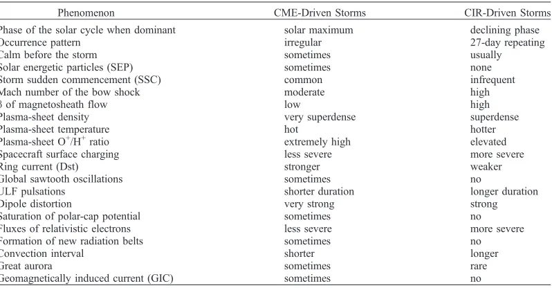
Differences between CME driven storms and CIR driven storms

Differences between CME-driven storms and CIR-driven storms

Joseph E. Borovsky1 and Michael H. Denton1,2

Received 28 September 2005; revised 27 February 2006; accepted 17 March 2006; published 26 July 2006.

[1] Twenty one differences between CME-driven geomagnetic storms and CIR-driven

geomagnetic storms are tabulated. (CME-driven includes driving by CME sheaths, by magnetic clouds, and by ejecta; CIR-driven includes driving by the associated recurring high-speed streams.) These differences involve the bow shock, the magnetosheath, the radiation belts, the ring current, the aurora, the Earth’s plasma sheet, magnetospheric convection, ULF pulsations, spacecraft charging in the magnetosphere, and the saturation of the polar cap potential. CME-driven storms are brief, have denser plasma sheets, have strong ring currents and Dst, have solar energetic particle events, and can produce great auroras and dangerous geomagnetically induced currents; CIR-driven storms are of longer duration, have hotter plasmas and stronger spacecraft charging, and produce high fluxes of relativistic electrons. Further, the magnetosphere is more likely to be

preconditioned with dense plasmas prior to CIR-driven storms than it is prior to CME-driven storms. CME-driven storms pose more of a problem for Earth-based electrical systems; CIR-driven storms pose more of a problem for space-based assets.

Citation: Borovsky, J. E., and M. H. Denton (2006), Differences between CME-driven storms and CIR-driven storms,J. Geophys. Res.,111, A07S08, doi:10.1029/2005JA011447.

1. Introduction

[2] CME-driven and CIR-driven geomagnetic events dif-fer, with the various forms of geomagnetic activity (ring current, aurora, convection, radiation belts,. . .) being man-ifested to different degrees in the two types of storms. In this paper a systematic comparison between the properties of CME-driven storms and CIR-driven storms is summarized. As will be seen, there are a large number of differences.

[3] It is not surprising that the two types of geomagnetic storms differ because the two types of drivers differ. Geomagnetic activity is chiefly driven by the value of vBs of the solar wind [e.g.,Bargatze et al., 1986], where v is the solar wind speed and Bsis the southward component of the interplanetary magnetic field (in GSM coordinates). For CME drivers and CIR drivers, many things differ: the strength and morphology of the magnetic field, the temporal profile of the velocity v, the durations of the vBsdrivers, the presence of shocks, . . . [e.g., Gonzalez et al., 1999]. Coronal mass ejections (CMEs) are preceded in time by a sheath of compressed solar wind, which itself is often preceded by an interplanetary shock. The strong magnetic field of the sheath can drive storms as well as can a strong magnetic field in the ejecta, and the interplanetary shock can add phenomenology to the geomagnetic storm on Earth. Additionally, the ejecta may contain a magnetic cloud. In this paper, CME-driven storms will refer to storms driven by all or some of the various components: shock, sheath,

ejecta, and cloud. Corotating interaction regions (CIRs) are followed in time by high-speed streams. Either the CIR or the high-speed stream or both can be drivers of storms. In this paper, CIR-driven storms refers to storms driven by either or both the CIR and the stream.

[4] The occurrence rate of CMEs peaks strongly during solar maximum [Webb, 1991; Yashiro et al., 2004], so storms during solar maximum tend to be CME-driven storms [Richardson et al., 2001]. The occurrence rate of well-formed CIR (with 27-day recurrence) peaks during the late declining phase of the solar cycle [Mursula and Zeiger, 1996], so storms in the declining phase tend to be CIR driven [Richardson et al., 2001]. Note that interaction regions (IRs) produced by nonrecurrent high-speed streams can occur throughout the solar cycle [Bobrov, 1983; L. Jian, private communication, 2005] and can drive nonrecurring geomagnetic activity throughout the solar cycle [Richardson et al., 2000], although the geomagnetic events that they drive are weaker than the recurring events of the declining phase [Bobrov, 1983].

[5] This study is a follow on to the multispacecraft study of Denton et al. [2006] which separately examined the magnetosphere’s reaction to the passage of CMEs and CIRs. In that study, superposed epoch intervals of various quan-tities measured by spacecraft in the magnetosphere were constructed using the peak negative Dst as the zero epoch. Six of the differences listed in Table 1 are findings of the Denton et al. superposed epoch study. The Denton et al.

[2006] study is itself a follow-up to aDenton et al.[2005] study in which the magnetospheric evolution during 283 geomagnetic storms was examined.

[6] The differences between CME-driven storms and CIR-driven storms are collected into Table 1. The differ-ences are discussed individually in section 2. For some Here

for Full Article

1

Los Alamos National Laboratory, Los Alamos, New Mexico, USA. 2_{Also at Department of Physics and Astronomy, University of} Southampton, Southampton, UK.

other properties of storms the differences could not be discerned within the scope of the present study; those phenomena are briefly discussed in section 3. The findings are summarized in section 4.

2. Differences

[7] The differences between CME-driven storms and CIR-driven storms are collected into Table 1. The category ‘‘CME-driven’’ includes driving by ejecta, CME sheaths, and magnetic clouds. The category ‘‘CIR-driven’’ also includes driving by the high-speed-stream that follows the CIR. Each row of Table 1 is described in detail in the various subsections of this section. For some storm proper-ties, the differences between CME-driven storms and CIR-driven storms are well known and the appropriate literature is pointed out. For other properties, original work is done here to discern the differences.

2.1. Phase of the Solar Cycle

[8] It is well known that CIR-driven storms generally occur in the late declining phase of the solar cycle and that CME-driven storms tend to occur at solar maximum [Gonzalez et al., 1999; Yermolaev and Yermolaev, 2002;

Richardson et al., 2001, 2002]. There are exceptions to this general trend. CMEs occur throughout the solar cycle, but their occurrence frequencies and their velocities are both greatest during solar maximum [Webb and Howard, 1994;

Ivanov and Obridko, 2001;Gopalswamy et al., 2004]. Also, 27-day-recurring high-speed streams can also occur in phases of the solar cycle other than the declining phase. Additionally, interaction regions (IRs) that are not 27-day recurring occur throughout the solar cycle [Bobrov, 1983;Richardson et al., 2000], although their geomagnetic effectiveness is weaker on average than is the geoeffectiveness of CIRs.

2.2. Occurrence Rate

[9] CIRs (corotating interaction regions), when they oc-cur, pass the Earth every27 days owing to the rotation of

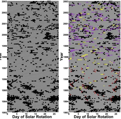
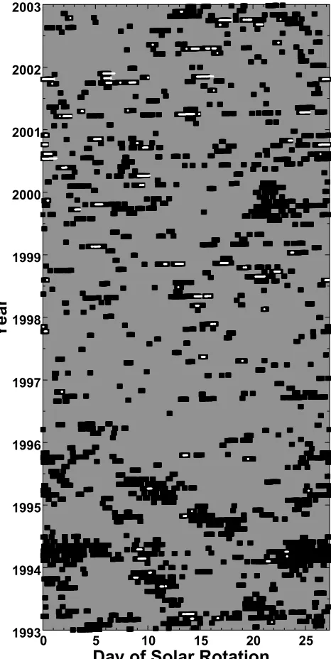
the Sun. During the declining phase of the solar cycle, coronal hole structure on the solar surface is long-lived and simple, and as a result 27-day-recurring high-speed-stream-driven storms are often found. This is shown in Figure 1a. Here the Kp index is used to create a storm occurrence database. The Kp index is broken into 27.27-day-long intervals, one interval for each rotation of the Sun. The data is then plotted as the day during the 27.27-day-long interval (horizontal) versus the fractional year (vertical). The timelines are the thin black lines. Time intervals when Kp4+are plotted as large black squares. 27-day repeating storms appear as the vertical clusters of black points. Several of these storm groups can be seen in 1993 – 1995 during the declining phase. Another group can be seen in late 1999 and early 2000. The storms are replotted in Figure 1b without the timeline. The McPherron online catalog (R. McPherron, private communication, 2005) (www.igpp.ucla.edu/public/rmcpherr/CDAWEventLists/) of CIR stream interfaces at Earth for January 1994 through December 1996 is used to produce the yellow points in Figure 1b. As can be seen by their association with CIRs, the groups of periodic storms in Figure 1a are high-speed-stream-driven storms (CIR-driven storms). As can be seen in Figure 1a, throughout the solar cycle other storms occur randomly. The occurrence frequency of these random storms is higher in the 2000 – 2002 solar maximum years. Plotted in purple in Figure 1b are times when CMEs are passing the Earth (the Cane and Richardson catalog [Cane and Richardson, 2003]) and plotted in yellow are times when magnetic clouds are passing the Earth (the Lepping online catalog http://lepmfi.gsfc.nasa.gov/mfi/mag_cloud_pub1. html, seeLepping et al.[2005]). The Cane and Richardson catalog goes from January 1996 through December 2002 and the Lepping catalog goes from February 1995 through August 2003. As can be seen, the randomly occurring storms in Figure 1a are associated with CMEs and with the magnetic clouds within CMEs.

Table 1. A Summary of Some of the Important Differences Between CME-Driven Storms (Shock, Sheath, Ejecta, Cloud) and CIR-Driven Storms (CIR, High-Speed Stream)

Phenomenon CME-Driven Storms CIR-Driven Storms

Phase of the solar cycle when dominant solar maximum declining phase

Occurrence pattern irregular 27-day repeating

Calm before the storm sometimes usually

Solar energetic particles (SEP) sometimes none

Storm sudden commencement (SSC) common infrequent

Mach number of the bow shock moderate high

bof magnetosheath flow low high

Plasma-sheet density very superdense superdense

Plasma-sheet temperature hot hotter

Plasma-sheet O+/H+ratio extremely high elevated

Spacecraft surface charging less severe more severe

Ring current (Dst) stronger weaker

Global sawtooth oscillations sometimes no

ULF pulsations shorter duration longer duration

Dipole distortion very strong strong

Saturation of polar-cap potential sometimes no

Fluxes of relativistic electrons less severe more severe

Formation of new radiation belts sometimes no

Convection interval shorter longer

Great aurora sometimes rare

2.3. Calm Before the Storm

[10] Borovsky and Steinberg [2006] found that most recurring high-speed-stream-driven storms have an extended interval (1 – 2 days) of extreme geomagnetic calm (Kp1+) within 24 hours prior to storm onset. These calms before the storms are caused by the same Russell-McPherron effect that produces an increased probability of high-speed-stream-driven-storm occurrence [cf. Crooker and Cliver, 1994;

Mursula and Zeiger, 1996]: owing to a sector reversal just upstream of the CIR stream interface, when the IMF in the high-speed wind is favorable for a storm, the IMF in the slow wind is favorable for a calm. A survey of 83 high-speed-stream-driven storms by Borovsky and Steinberg

[2006] found that 67% of the storms were immediately preceded by extended intervals of geomagnetic calm. Using the same analysis techniques, a survey by the present authors of 68 CME-driven storms (from the Denton et al. [2006]

catalog) finds that only 37% are immediately preceded by extended intervals of calm. Hence calms before the storms are predominantly a CIR-driven-storm phenomena. Calms before storms are of note because during the calm intervals the magnetosphere fills with dense plasmaspheric plasma and with dense LLBL (low-latitude boundary layer) plasma. The buildup of dense plasma in the magnetosphere can change the nature of a storm, yielding a stronger ring current (B. Lavraud et al., Magnetosphere preconditioning under northward IMF: Evidence from the study of CME and CIR geoeffectiveness, submitted to Journal of Geophysical Research, 2006), initially lower fluxes in the outer radiation belts [Borovsky and Steinberg, 2006], and perhaps changes to the reconnection rate at the dayside neutral line [Borovsky and Steinberg, 2006]. CIR-driven storms are more often preconditioned by calms than are CME-driven storms.

2.4. Solar Energetic-Particle (SEP) Events

[11] Solar energetic-particle events are enhanced fluxes of subrelativistic and relativistic ions that have durations of hours to days. SEP events are well known to be associated with solar flares and with strong interplanetary shocks driven by ejecta from the sun [Reames, 2003]. Flares and strong interplanetary shocks are both phenomena that are associated with CMEs, hence SEP events sometimes ac-company CME-driven storms. The intensity of SEP events is correlated with the velocity of the coronal ejecta driving the shocks [Kahler, 2001]. On rare occasions, SEP events can be large enough to pose a hazard to aircraft passengers

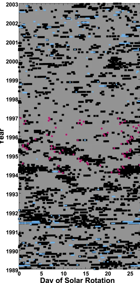
and electronics [Dyer et al., 2003] and to astronauts in high-latitude orbits [Reames, 1999a]. Energetic-particle events are also produced by CIRs (by CIR shocks in the helio-sphere beyond2 AU, with the energetic particles traveling back to 1 AU) [Reames, 1999b], but their intensity at Earth is weak compared with CME-related SEP events [Mason and Sanderson, 1999], extending only to20 MeV/n. In Figure 2 it is demonstrated that major SEP events often accompany CME-driven storms and are not associated with CIR-driven storms. Here, for the years 1989 – 2003, storms (black boxes) are displayed in a solar-rotation versus time plot. The NOAA online SEP-event catalog (http://www.sec.noaa.gov/ftpdir/indices/SPE.txt) is plotted as the blue points. These events have integral fluxes of >10 MeV protons at geosynchronous orbit that exceed 10 protons/cm2/s/ster. As can be seen, there are large numb-ers of SEP events among the storms during the two solar maxima in the figure (the years 1989 – 1992 and 2000 – 2002) but there are no SEP events associated with the 27-day-recurring storm groups in the years 1993 – 1995 nor in the 27-day-recurring storm group in late 1999/early 2000. Also plotted in pink in Figure 2 is the McPherron catalog of CIR stream interfaces for the years 1994 – 1996. As can be seen, there is at most one SEP event that is associated with one of the 74 CIRs in the catalog, and this SEP is flare associated.

2.5. Storm Sudden Commencement (SSC)

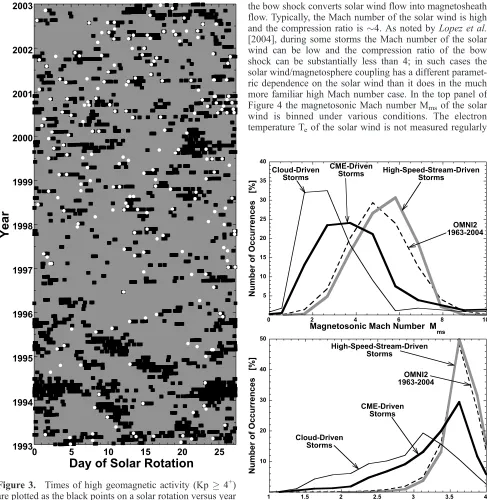
[12] Most storm sudden commencements are associated with strong interplanetary shocks that compress the magne-tosphere [Iucci et al., 1988;Russell et al., 1992]. The strong shocks are usually found ahead of fast CMEs. As pointed out byKamide et al. [1998], CIR-driven storms generally lack sudden commencements [see alsoVenkatesan and Zhu, 1991]. An examination of storms by Taylor et al. [1994] supports the conclusion that SSCs tend to be driven by CMEs, with more gradual onsets being driven by high-speed streams. In Figure 3, SSCs (white circles) and storms (black boxes) are displayed on a solar rotation versus time plot. The SSCs are from the NOAA online SSC catalog (http://www.ngdc.noaa.gov/stp/SOLAR/ftpSSC.html). As can be seen in the figure, SSCs tend to not be associated with the groups of 27-day-recurring storms (cf. the years 1993, 1994, 1995, and 1999). Also, as can be seen in the figure, SSCs are associated with the randomly occurring storms. To quantify these observations, the Borovsky and Steinberg [2006] catalog of high-speed-stream-driven storms is examined and it is found that 21% of those storms are temporally associated with SSCs from the NOAA SSC catalog. Forming a CME-driven-storm catalog by requiring Kp4+in theCane and Richardson[2003] CME catalog and the Lepping online [Lepping et al., 2005] magnetic cloud catalog, it is found that 69% of those CME-driven storms are temporally associated with SSCs from the NOAA SSC catalog. Hence SSCs are common (70%) for CME-driven storms and infrequent (20%) for CIR-driven storms.

2.6. Magnetosonic Mach Number of the Solar Wind [13] Depending on the values of the Alfven velocity vA= B/(4pnmi)1/2and ion-acoustic speed Cs= (kB(Ti+ Te)/mi)1/2 in the solar wind, the magnetosonic Mach number Mms = vsw/(vA2 + 5Cs2/3)1/2 of the solar wind flow relative to the Figure 2. Times of high geomagnetic activity (Kp4+)

Earth can change. The magnetosonic Mach number Mms sets the properties of the bow shock, which converts unshocked solar wind plasma into shocked magnetosheath plasma. The magnetosonic Mach number controls the compression ratio C of the shock, which is the multiplica-tive density change from upstream to downstream. The compression ratio C varies from 1 (at Mms = 1) to 4 (at Mms ! 1) [Tidman and Krall, 1971]. In solar wind/ magnetosphere coupling, it is actually the magnetosheath flow that drives activity in the Earth’s magnetosphere, and

the bow shock converts solar wind flow into magnetosheath flow. Typically, the Mach number of the solar wind is high and the compression ratio is4. As noted byLopez et al.

[2004], during some storms the Mach number of the solar wind can be low and the compression ratio of the bow shock can be substantially less than 4; in such cases the solar wind/magnetosphere coupling has a different paramet-ric dependence on the solar wind than it does in the much more familiar high Mach number case. In the top panel of Figure 4 the magnetosonic Mach number Mmsof the solar wind is binned under various conditions. The electron temperature Teof the solar wind is not measured regularly

Figure 3. Times of high geomagnetic activity (Kp4+) are plotted as the black points on a solar rotation versus year plot. Times of occurrence of SSCs (storm sudden commencements) at Earth are indicated which white circles. The SSCs occurrence times are from the NOAA online SSC c a t a l o g ( h t t p : / / w w w. n g d c . n o a a . g o v / s t p / S O L A R / ftpSSC.html).

and hence is not available in the OMNI data sets, so to calculate the ion acoustic speed Cs= (kB(Ti+ Te)/mi)1/2of the solar wind, Te= 1.5105K = 12.9 eV is taken, which is approximately valid for all types of solar wind [Skoug et al., 2000]. All other solar wind parameters are obtained from the OMNI2 solar wind data set [King and Papitashvili, 2005]. The dashed curve in Figure 4 is the occurrence distribution of magnetosonic Mach numbers in the entire 1963 – 2004 OMNI2 data set. The thick gray curve is the occurrence distribution for times when stream-driven storms are ongoing. The collection of high-speed-stream-driven-storm times is the Borovsky and Steinberg

[2006] catalog of storms driven by 27-day recurring high-speed streams. As can be seen, the Mach numbers during high-speed-stream-driven storms have a typical distribution of values (i.e., similar to OMNI2). The thick black curve in Figure 4 is for times when CME-driven storms are ongoing and the thin black curve is for times when the magnetic clouds are passing during CME-driven storms. The collec-tion of CME-driven-storm times is obtained by requiring Kp4+in the Cane and Richardson[2003] CME catalog and the collection of cloud-driven storm times is obtained by requiring Kp4+in the Lepping online magnetic cloud catalog [cf.Lepping et al., 2005]. As can be seen, the Mach numbers of the solar wind are anomalously low for CME-driven storms and even lower for the cloud-CME-driven storms. In the bottom panel of Figure 4, the compression ratio C across the bow shock is binned for the same conditions as in the top panel. The compression ratio for the bow shock is estimated using the Rankine-Hugoniot shock jump condi-tions (equacondi-tions (1.50) and (1.51) of Tidman and Krall

[1971]) under the assumption of a quasi-perpendicular shock. The dashed curve in the bottom panel is the occurrence distribution of C for the entire 1963 – 2004 OMNI2 data set. As can be seen, the compression ratio C is typically near 4. The thick gray curve in the bottom panel is the distribution of C values for times when high-speed-stream-driven storms are ongoing; as can be seen C is typically near 4 for high-speed-stream-driven storms. The thick black curve in the bottom panel is for times when CME-driven storms are ongoing and the thin black curve is for the magnetic cloud portions of CME-driven storms. As can be seen, the bow shock compression ratio for CME-driven storms, and particularly for cloud-CME-driven storms, is not near 4. For cloud-driven storms, 26.8% of the time C is less than 2.5, which is the midway point between the limits of 1 and 4. Because of the systematic difference in the bow shock compression ratio, it is expected that the dependence of geomagnetic activity on solar wind parameters will differ for CME-driven and high-speed-stream-driven storms.

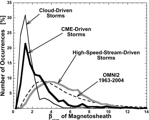
2.7. Plasma-Bof the Magnetosheath

[14] For the solar wind parameters that lead to global sawtooth oscillations of the magnetosphere, it has been noted that the plasma-b value of the magnetosheath is anomalously low [Borovsky, 2004; J. E. Borovsky et al., The solar-wind driving of global sawtooth oscillations and periodic substorms: What determines the periodicity?, sub-mitted toAnnales Geophysicae, 2006, hereinafter referred to as Borovsky et al., submitted manuscript, 2006], often less than unity. The plasma-b is a measure of how strongly distorted the magnetic field can be owing to diamagnetic

currents in the plasma.bcan be defined two ways: a thermal

bdefined asbth= 8pnkB(Ti+ Te)/B2or a rambdefined as

bram = 4pnmiv2/B2 where v is the plasma flow velocity [Parsons and Jellison, 1983; Borovsky, 1992]. bth is a measure of the currents when a warm plasma is confined by a magnetic field;bramis a measure of the currents when a plasma flow is deflected or slowed. Althoughbthbramin the magnetosheath plasma, we are specifically interested in the value of bram, which is the ratio of the ram pressure nmiv2 of a flow to the magnetic-field pressure B2/8p of the plasma. (Note also that bram = MA2, where MA is here the Alfven Mach number of the magnetosheath flow.) If

bram < 1, a flow has difficulty distorting magnetic-field lines. Ordinarily, in the magnetosheath bram 1 and the flow of the magnetosheath is little impeded by the magnetic field in the magnetosheath. In that case a gasdynamic flow picture [e.g., Alksne and Webster, 1970; Spreiter and Stahara, 1994; Stahara, 2002] is valid with the magnetic field lines passively convected by the magnetosheath flow; strong draping of the field lines over the magnetosphere results. Global MHD simulations of the solar-wind-driven magnetosphere whenbram< 1 in the magnetosheath [Borovsky et al., 2004] find that the magnetosheath mag-netic field lines are stiff and do not drape; the stiff field lines squeeze the magnetosphere into an unusual flattened shape and produce an asymmetric magnetosheath flow pattern that is very different from the gasdynamic picture. Thebram of the magnetosheath flow can be estimated from upstream solar wind parameters by using the Rankine-Hugoniot quasi-perpendicular shock jump conditions. Taking Te = 12.9 eV for the solar wind (see section 2.6) along with measured values of v, Ti, B, and n in the solar wind, equations (1.50) and (1.51) of Tidman and Krall [1971] yieldbramvalues for the magnetosheath plasma. In Figure 5 Figure 5. For various data sets (as labeled) the

plasma-bram value of the magnetosheath estimated from the Rankine-Hugoniot shock-jump conditions and upsteam solar wind parameters is binned. The median values of

these bram values are binned for various conditions. The dashed curve is the occurrence distribution of bram for the entire 1963 – 2004 OMNI2 data set. As can be seen from the OMNI2 curve, bram in the magnetosheath is typically high. The thick gray curve is for times when high-speed-stream-driven storms are ongoing, the thick black curve is for times when CME-driven storms are ongoing, and the thin black curve is for times when magnetic clouds are passing the Earth during storms. As can be seen, for high-speed-stream-driven stormsbramis slightly higher than typical. Thebram values for CME-driven storms are anomalously low and the

bramvalues for the magnetic cloud portions of CME-driven storms are even lower. For the OMNI2 data set, 0.75% of the timebram< 1 in the magnetosheath. For high-speed-stream-driven storms, only 0.17% of the time isbram< 1, whereas for CME-driven storms 8.14% of the timebram< 1 and for cloud-driven storms 24.1% of the timebram< 1.

2.8. Plasma Sheet Density

[15] The density of the Earth’s plasma sheet is gov-erned by the solar wind density with a few hour time lag [Borovsky et al., 1998a]. In a superposed epoch study,

Denton et al. [2006] compared the Earth’s plasma sheet density for CME-driven storms with its density for CIR-driven storms as functions of time during the storm and local time around geosynchronous orbit. Typical nonstorm nightside densities are 0.7 cm3. For both CME-driven and CIR-driven storms, Denton et al. found that super-dense plasma sheets [cf. Borovsky et al., 1997] occur, with the density being twice or more the typical value. In comparing the two drivers, CMEs drive a plasma sheet that is more dense and the high-density values persist longer. The relatively brief superdense intervals in CIR-driven storms appear to coincide with the CIR, which has a high solar wind density; this is in contrast to the enhanced geomagnetic activity, which persists long into the high-speed stream that follows the CIR. This is because high-speed streams have only modest densities although they have strong vBz. In a similar fashion, the superdense intervals of CME-driven storms probably coincide with the passing of the higher-density CME sheath. Note that CME-driven storms without a super-dense plasma sheet can occur [e.g., Thomsen et al., 1998a; Seki et al., 2005].

2.9. Plasma Sheet Temperature

[16] In a superposed epoch study, Denton et al. [2006] compared the Earth’s plasma sheet ion and electron temperatures for CME-driven storms with CIR-driven storms, making the examination as functions of time during the storm and local time of the spacecraft mea-surement. For both types of storms the ion and electron temperatures are substantially elevated over typical val-ues, probably because the solar wind speed is high and the plasma sheet temperature is related to the solar wind velocity [Borovsky et al., 1998a]. Comparing the plasma sheet temperature for the two types of storms (Figure 4 of Denton et al.), the plasma sheet is hotter for the CIR-driven storms than it is for the CME-CIR-driven storms and the elevated temperatures persist longer (days) for CIR-driven storms. This is particularly evident when the electron temperatures are examined.

2.10. Plasma Sheet Composition

[17] In the superposed epoch study,Denton et al.[2006] compared the estimated O+/H+ ratio in the Earth’s plasma sheet for CME-driven storms with CIR-driven storms as functions of time during the storm and local time around geosynchronous orbit. Both types of storms produced elevated ratios, but CMEs that drive large Dst storms producing very elevated O+/H+ ratios (exceeding unity). Hence CME-driven storms can have very strong iono-spheric outflows of O+and CME-driven storms can produce plasma sheets that are predominantly O+by number density.

2.11. Spacecraft Surface Charging

[18] In the superposed epoch study,Denton et al.[2006] compared the measured voltages of geosynchronous-orbit spacecraft with respect to the ambient plasma for CME-driven storms with CIR-CME-driven storms. The comparison is made as functions of time during the storm and local time of the spacecraft. For both types of storms the hot plasmas of the magnetosphere drive substantial spacecraft charging, even outside of the Earth’s shadow. The spacecraft charging that occurs during CIR-driven storms is more severe than it is for CME-driven storms: the voltages attained are higher (greater than 1000 volts), the region of local time over which the severe charging occurs is wider across the nightside of the magnetosphere, and the high voltages persist longer (days). This result is consistent with the well-known fact that spacecraft charging is driven by hot electrons [Whipple, 1981; Mullen et al., 1986], and, as discussed in section 2.5 above, the electron temperatures of the magnetosphere are hotter and more persistent for CIR-driven storms than they are for CME-driven storms. Note that voltages of differential surface charging of space-craft are proportional to the voltages of surface charging [cf.

Borovsky et al., 1998b, Figure 10], so differential surface charging is anticipated to be more severe during CIR-driven storms than it is during CME-driven storms.

2.12. Ring Current and Dst

[19] In a survey of Dst perturbations, Yermolaev and

Yermolaev [2002] found that CMEs are more effective at producing strong Dst values than are CIRs and high-speed streams. This conclusion is borne out by theDenton et al.

makes sense that Dst is stronger for CME-driven storms than it is for CIR-driven storms.

2.13. Global Sawtooth Oscillations

[20] Global sawtooth oscillations are periodic (3 – 4 hours) oscillations of the magnetosphere that are characterized by a slow global distortion of the magnetosphere followed by a rapid crash back to a less-distorted morphology [Borovsky et al., 2001]. They are observed to be driven by magnetic clouds in CMEs that have southward magnetic field in the range of 5 to15 nT and that tend to have parameters that lead to polar cap saturation (Borovsky et al., submitted manuscript, 2006). This is low Mach number solar wind and for these parameters the Earth’s magnetosheath is a b < 1 plasma,

which has very unusual flow properties (see section 2.7). Why these solar wind conditions lead to sawtooth oscillations of the magnetosphere during storms is presently an area of active research. Global sawtooth oscillations are not seen during CIR-driven storms (Borovsky et al., submitted manuscript, 2006).

2.14. ULF Pulsations

[21] ULF oscillations in the magnetosphere have been reported for CME-driven storms [Baker et al., 1998] and high-speed-stream-driven storms [Kessel et al., 2004], with pulsation activity peaking in the declining phase of the solar cycle [Zieger, 1991]. In Figure 7 the power of ULF pulsations PULF in the dawnside magnetosphere is binned for various conditions. The data set used is the 1987 – 2000 daily average of the dawnside power obtained from the IMAGE and SAMNET ground-based magnetometer net-works, courtesy of P. O’Brien (private communication, 2005); a description of the data set is found in the work ofO’Brien et al.[2003]. The dashed curve is the occurrence distribution of Log10(PULF) for the entire 1987 – 2000 PULF data set. The thick gray curve is the occurrence distribution of Log10(PULF) during high-speed-stream-driven storms, the thick black curve is the occurrence distribution of Log10 (PULF) during CME-driven storms, and the thin black curve is the occurrence distribution of Log10(PULF) during the magnetic cloud portions of CME-driven storms. As can be seen in Figure 7, PULF is elevated above normal for all types of storms. The amplitude of Pc5 oscillations in the magnetosphere is proportional to the solar wind velocity [Engebretson et al., 1998;Mathie and Mann, 2001]. Elec-tron acceleration by Pc5 oscillations are believed to be responsible for the production of high fluxes of relativistic electrons in the outer radiation belts [Rostoker et al., 1998], particularly during long intervals of active ULF pulsations [Mathie and Mann, 2000; O’Brien et al., 2001], which

Figure 6. Times of high geomagnetic activity (Kp4+) are plotted as the black boxes on a solar rotation versus year plot. Times when Dst <100 are plotted as white points.

occur during longer intervals of high-velocity solar wind associated with recurrent high-speed streams. This is shown in Figure 8, where storms and intervals of high ULF power are shown on a solar rotation versus time plot for the years 1987 – 2000. The storms are indicated as black boxes and intervals when PULF > 1 107 nT2/Hz are indicated as white circles. As can be seen, the longest (multiday) inter-vals of elevated ULF power are found with the 27-day recurring storm groups, particularly in the year 1994. The intervals of active ULF pulsations are longer for CIR-driven storms than they are for CME-CIR-driven storms because the intervals of elevated solar wind velocity are longer.

Evidence for this can be found in Figure 9. For full years when there is thorough data coverage of the solar wind (the years 1995 – present), a measure of the duration of high-speed flows is plotted in Figure 9 as the green bars. This measure is made as follows. For each year of data, the durations of all flows wherein the solar wind velocity is sustained at 550 km/s or higher are calculated. Then, for each year, the 12 longest-duration fast flows are taken. The height of the green bar in Figure 9 is the mean duration for those 12 longest flows that year. The sunspot number is also plotted as the black bars in Figure 9, and intervals when 27-day recurring storms (which are high-speed-stream driven) were ongoing are marked with the horizontal blue bands (see section 2.2 for the methodology of finding the recurring storm groups). As can be seen, when recurring CIR-driven storms were ongoing (which tends to be in the declining phase of the solar cycle), the fast flow durations were longer. Since the power in ULF pulsations is propor-tional to the solar wind speed, it follows that the duration of intervals of enhanced ULF activity are longer in years when CIR-driven storms are present than for the rest of the solar cycle. This is also shown in Figure 9, where a 0.5-year running average of the measured flux of 1.1 – 1.5 MeV electrons at geosynchronous orbit is plotted as the red curve. (See section 2.17 for a description of this measurement.) This flux is elevated in the years when the durations of the high-speed flows were long (green bars).

2.15. Distortion of the Dipole

[22] CIR-driven storms produce modest stretching of the dipole magnetic field toward a tail-like geometry (with the near-equatorial field at geosynchronous orbit rotated30

Figure 8. Times of high geomagnetic activity (Kp4+) are plotted as the black boxes on a solar rotation versus year plot. Times when the dawnside ULF power PULF exceeds 1107nT2/Hz are plotted as white circles. The ULF power was provided by Paul O’Brien [O’Brien et al., 2003].

from dipolar) with the stretching angle proportional to the local pressure of the ion plasma sheet [seeBorovsky et al., 1998b, Figure 18]. During times when global sawtooth oscillations occur, which are driven by CMEs, the dipole magnetic field can show fully tail-like stretching at geosyn-chronous orbit (with the near-equatorial field rotated70

from dipolar) (Borovsky et al., submitted manuscript, 2006). Two further studies indicate that large distortions of the dipole magnetic field are associated with CME-driven storms. First, the Tsyganenko et al. [2003] catalog of big distortion events for the inner magnetosphere all were large Dst events that occurred at solar maximum, which is indicative of driving by CMEs. Second, the flankside lobe encounters by geosynchronous spacecraft at the equator that were tabulated during an interval of solar maximum found that most lobe encounters were associated with large-Dst storms [Moldwin et al., 1995], which is also consistent with driving by CMEs.

2.16. Saturation of Polar Cap Potential

[23] Typically, under vBs driving by the solar wind, the cross-polar-cap potential j is linearly proportional to vBs [Reiff and Luhmann, 1986], where v is the solar wind velocity and Bsis the southward (GSM) component of the IMF, but under rare circumstances when the solar wind conditions are favorable, the cross-polar-cap potentialjwill reach a saturation value and will no longer be proportional to vBs. During several CME-driven storms this saturation has been analyzed [Ober et al., 2003; Boudouridis et al., 2004; Hairston et al., 2005]. Equation (1) of Siscoe et al.

[2004] describes this saturation: saturation occurs when the second term in the denominator of that equation exceeds approximately 2, which occurs when

vASP=806>2; ð1Þ

where vAis the Alfven velocity in the unshocked solar wind (in units of km/s) andSP is the height-integrated Pederson conductivity of the dayside ionosphere (in units of mho). Taking SP = 0.77 F10.71/2 (from equation (4) of Ober et al. [2003]), where F10.7 is the radio emission of the Sun at 10.7 cm which is a proxy for solar EUV emission which produces ionospheric ionization [cf.Balan et al., 1993], and F10.7 SN (from Figure 1 and Table 2 of Floyd et al. [2005]), where SN is the international sunspot number, expression (1) is rewritten as

QvAS1N=2=1050>2; ð2Þ

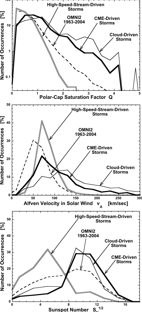
where Q is a saturation parameter. The OMNI2 data set is used to find times when expression (2) is satisfied: the results are displayed in Figures 10 and 11. In Figure 10 the temperature-speed plot of the solar wind using the OMNI2 data set [King and Papitashvili, 2005] is shown (black points) and the data points wherein expression (2) is satisfied are plotted in red. Expression (2) is satisfied 0.96% of the time in the 1963 – 2004 OMNI2 data set. These red points where the solar wind will drive the polar cap voltage into saturation are outliers to the normal solar wind population; this is consistent with the red points being CMEs [see, e.g.,Elliott et al., 2005, Figure 1a]. In Figure 11 the sunspot number SNis plotted as a function of time as the black points, with the values at times when expression (2) is satisfied plotted in red. As can be seen, the time intervals when expression (2) is satisfied occur during solar maxima; this is again consistent with those times being CMEs. A detailed examination of ACE solar-wind data for time intervals when expression (2) is satisfied (J. Steinberg, private communication, 2005) finds that most of those intervals are in CMEs, typically CMEs with low number density. A minor fraction of the points in the OMNI2 data set satisfying expression (2) are low-density pressure balance structures embedded in the solar wind. Polar cap Figure 10. Using the hourly averaged solar wind values in

the 1963 – 2004 OMNI2 data set, the ion temperature of the solar wind is plotted as a function of the velocity of the solar wind (black points). During time intervals when the conditions of the solar wind should result in a saturation of the Earth’s cross-polar-cap potential (expression (2)), the points are replotted in red. As can be seen, the red points form a population of outliers around the main solar wind population.

saturation is usually thought of as a phenomenon associated with strong storms, but note that according to expression (2) and Figure 10 the polar cap potential will saturate for drivers that are not extremely strong (i.e., it will saturate for slow CMEs also). To further explore the polar cap saturation for CME- and CIR-driven storms, the value of Q is binned under various circumstances in the top panel of Figure 12. The dashed curve is the occurrence distribution of Q for the entire 1963 – 2004 OMNI2 data set, the thick gray curve is the occurrence distribution of Q for high-speed-stream-driven storms, the thick black curve is the occurrence distribution of Q for CME-driven storms, and the thin black

curve is the occurrence distribution of Q for the magnetic cloud portions of CME-driven storms. As can be seen, saturation of the polar cap (Q > 2) occurs rarely for high-speed-stream-driven storms but commonly for CME-driven storms. Even considering partial saturation, for high-speed-stream-driven storms only 4.4% of the time is Q > 1, whereas for CME-driven storms 39.3% of the time Q > 1 and for cloud-driven storms 54.2% of the time Q > 1. To explore whether the polar cap saturation is simply owed to the high values ofSP during solar maximum when CMEs tend to occur, the Alfven velocity vAin the solar wind and the square root of the sunspot number SN1/2are binned in the middle and bottom panels of Figure 12. Examining the various curves in the middle and bottom panels it can be concluded that the higher values of Q = vASP/806 = vASN1/2/ 1050 for CME-driven storms are owed both to higher values of vAin the solar wind and to higher values of SN1/2.

2.17. Fluxes of Relativistic Electrons

[24] The Earth’s outer electron radiation belt is very dynamic. It is well known that the fluxes of relativistic electrons in the outer radiation belt are maximized by recurring high-speed-stream-driven storms during the de-clining phase of the solar cycle [Paulikas and Blake, 1976;

Love et al., 2000; Lam, 2004]. Sufficiently high fluxes of electrons in this belt lead to internal charging in spacecraft, which leads to operational problems for spacecraft in geosynchronous orbit [Romanova et al., 2005]. The fre-quency of these problems peaks during the declining phase of the solar cycle where CIR-driven storms peak [Wrenn et al., 2002]. In Figure 13 the production of intense fluxes of relativistic electrons in the outer radiation belts by the two types of storms in explored. For the years 1993 – 2001 geomagnetic storms are indicated (black boxes) on a solar rotation versus time plot. The 27-day-recurring storm groups (CIR-driven storms) are clearly seen in 1994 and 1995 and in late 1999/early 2000. The McPherron catalog of CIR stream interfaces for the years 1994 – 1996 is plotted in yellow. In Figure 13, times when the multispacecraft daily average of 1.1 – 1.5 MeV electrons at geosynchronous orbit as measured by the SOPA energetic particle instru-ments [Belian et al., 1992] exceeds 30 electrons/cm2/s/ster/ keV are indicated in red. The relativistic-electron fluxes

were provided by R. Friedel (private communication, 2005). As can be seen in the figure, the high fluxes of relativistic electrons are predominantly associated with CIR-driven storms. There are some relativistic electron events that are associated with randomly occurring storms, e.g., in the years 1996 – 2002, but a comparison of these events with the Cane and Richardson CME catalog and the Lepping magnetic cloud catalog finds that only one event is clearly CME related. It may be that the nonrecurrent relativistic electron flux events are associated with IRs (i.e.,

nonrecur-rent high-speed-stream-driven storms). In Figure 13, note the well-known delay in the appearance of intense relativ-istic electron fluxes from the onsets of the storms [cf.

Friedel et al., 2002].

2.18. Formation of New Ion and Electron Radiation Belts

[25] The production of a new ion radiation belt is known to be caused by the capture of SEP ions during a strong shock compression of the magnetosphere [Lorentzen et al., 2002; Hudson et al., 2004]. SEPs and strong shocks are both CME-driven phenomena, and the formation of a new ion radiation belt is therefore a manifestation of CME-driven storms. The formation of a new inner electron radiation belt has been observed coincident with the com-pression of the magnetosphere by SSCs [Blake et al., 1992;

Tverskaya et al., 2003;Obara and Li, 2003;Looper et al., 2005]. The mechanism is believed to be a displacement of trapped electrons during a rapid compression and relaxation of the magnetosphere caused by a CME-driven interplane-tary shock [Li et al., 1993]. No formation of a new radiation belt has been observed in association with a CIR.

2.19. Magnetospheric Convection Interval

[26] In the superposed-epoch study of the reaction of the magnetosphere to CMEs and CIRs, Denton et al. [2006] examined the temporal profile of the Kp index. Kp is a measure of the strength of convection in the magnetosphere [Thomsen, 2004]. Denton et al. found that CMEs produce a Kp temporal profile that is peaked near the time of Dst maximum and that falls quickly (in a fraction of a day) back to prestorm levels, whereas CIRs produce a Kp temporal profile that peaks near the time of Dst maximum but falls slowly (over a few days) back to prestorm levels. Hence the interval of enhanced convection is longer for CIR-driven storms than it is for CME-driven storms. This can also be seen in both panels of Figure 1, where the durations of the storms in the 27-day recurring groups (high-speed-stream-driven storms) is notably longer than the durations of the randomly occurring storms (CME-driven storms). Note that the maximum values of Kp, i.e., the strongest peak convec-tion, can be higher for CME-driven storms [e.g.,Richardson et al., 2001, Figure 1].

2.20. Great Aurora

[27] Great auroras have ‘‘high visual brightness with a progression to exceptionally low latitudes’’ [Jones, 1992]. An examination of the catalog of great aurora events of Jones [1992], supplemented by Yevlashin [2000],

Pallamraju and Chakrabarti [2005], and Mikhalev et al.

[2004], finds that the great aurora chiefly occur during solar maximum. A display of the solar cycle dependence of great aurora is shown in Figure 14, where the sunspot number is plotted as a function of time and the reported occurrences of great aurora are indicated by the circles. As can be seen, there is a concentration of great auroras at the solar maxima, but they occur in other phases in the solar cycle, too. In Figure 15 intervals of Kp4+(black points) and incidents of great auroras (tan points) are displayed on a 27.27-day solar-rotation versus year plot. Here, data for the 55 years 1950 – 2005 are shown. Recurrent storm activity (high-speed-stream-driven storms) is seen as a black patch. As Figure 13. Times of high geomagnetic activity (Kp4+)

can be seen, the great aurora generally are not associated with the recurrent activity, rather they are associated with isolated storms. Perusing through Figure 15 at high reso-lutions, two exceptions are found: 13 – 14 July 1982, where a great aurora incident occurred during a recurrent storm, and 13 September 1993, where a great aurora incident occurred during a recurrent high-speed stream. The July 1982 incident was flare-associated, so this major storm was likely CME associated. The September 1993 incident was not flare-associated and no solar wind data is available to discern whether or not a magnetic cloud was embedded in the high-speed wind; no SSC occurred, so if a cloud was present, it was not extraordinarily fast. From Figure 15 and the subsequent analysis it is concluded that 1 out of 44 incidents of great aurora (2%) are caused by CIR-driven storms. Of the four incidents of great aurora that occurred during the years of the McPherron CIR catalog (the years 1994 – 1996 and 2002 – 2003), none was temporally associated with CIRs. Of the 11 incidents of great aurora that occurred during the years when both the Cane and Richardson CME catalog and the Lepping magnetic cloud catalog were available (the years 1998 – 2002), 10 were temporally associated with CMEs (91%). Hence from all of this evidence it is concluded that great aurora are associated chiefly with CME-driven storms and rarely with CIR-driven storms. Supporting this notion, Jones [1974] points out a study finding that low-latitude aurora ‘‘can usually be associated with solar flares occurring 1 to 4 days earlier.’’ Also, Legrand and Simon [1988] examined the latitudes of CME-associated and CIR-associated (‘‘shock’’ and ‘‘stream’’) aurora and found that the stream-associated aurora did not progress equatorward beyond 56, whereas the CME-associated aurora did. Consistent with this, of the 26 low-latitude auroral events measured by STELAB in

1989 – 2004 [Shiokawa et al., 2005], only one event oc-curred during the 1993 – 1995 era of recurring high-speed streams. Since the aurora do not progress as far equatorward for CIR-driven storms, it may also follow that the polar-cap area does not get as large for CIR-driven storms as it can during CME-driven storms.

2.21. Geomagnetically Induced Currents (GIC) [28] Geomagnetically induced currents that are hazardous to Earth-based electrical power systems are believed to be caused by rapid intensification of ionospheric currents that

Figure 14. The sunspot number is plotted as a function of time. Occurrences of great aurora [from Jones, 1992;

Yevlashin, 2000; Pallamraju and Chakrabarti, 2005;

Mikhalev et al., 2004] are plotted as the circles with diamond centers.

can be driven by shock compression of the magnetosphere or by a substorm [Pulkkinen et al., 2005]. Of the four events in the catalog ofBoteler[2001], plus the March 1991 event [Bolduc, 2002], the April 2000 event [Pulkkinen et al., 2003], and the October 2003 event [Kappenman, 2005], all have occurred at solar maximum or in the early declining phase. This is demonstrated in Figure 16 where the sunspot number is plotted versus time with the seven GIC events indicated as the circles with diamonds. From direct solar wind measurements or from their temporal association with large solar flares, all seven of these GIC events are associ-ated with CME-driven storms. Examining their locations relative to storms on solar rotation versus time plots (see Figure 15), none of the GIC events are associated with 27-day recurring geomagnetic activity. Hence it is concluded that hazardous GIC are predominantly associated with CME-driven storms rather than CIR-driven storms.

3. Other Stormtime Differences

[29] Several stormtime phenomena have not been or could not be analyzed for inclusion in Table 1. Some of these pertain to observations of the ionosphere. It is hoped that the discussion of this section will motivate future research to clarify how these phenomena fit into CME-driven and CIR-CME-driven geomagnetic storms.

[30] Large equatorial bubbles, which appear in the topside ionosphere when Dst is increasing in magnitude [Huang et al., 2002;Basu et al., 2005], have been reported for many CME-driven magnetic storms [e.g., Huang et al., 2001;

Abdu et al., 2003; Basu et al., 2005]. Large equatorial bubbles do occur for Dst perturbations at solar minimum but at a much lesser rate than they do at solar maximum [Huang et al., 2002]. The bubbles are attributed to penetration electric fields associated with build up of the ring current: since ring current buildup is greater for CME-driven storms, one would expect the bubbles to be primarily a CME-driven storm phenomenon.

[31] SAPS (subauroral polarization stream) and SAID (subauroral ion drift) ionospheric flow streams are associ-ated with a deep penetration of the ion plasma sheet into the dipolar magnetosphere [Anderson et al., 1993; Garner et al., 2004]. SAPS and SAID events have been observed and analyzed for several CME-driven storms [e.g.,Foster et al., 1994; Garner et al., 2004; Foster and Vo, 2002], but no comparisons have been made for their occurrence probabil-ities and properties for CIR versus CME-driven storms.

[32] A recently discovered phenomenon is the disappear-ance of AKR (auroral kilometric radiation) during CME-driven storms coincident with the appearance of a superdense plasma sheet [Seki et al., 2005;Morioka et al., 2003]. The AKR-disappearance events in the literature are all associated with CME-driven storms, except the 11 January 1994 event, which corresponds to a superdense plasma sheet in a recurring CIR-driven storm. A comparison of the nature of the AKR disappearance for the hotter superdense plasma sheets of CIR-driven storms and the cooler superdense plasma sheets of CME-driven storms has not been made.

[33] The injection of cool dense plasma sheet (CDPS) material (which is probably low-latitude boundary layer (LLBL) plasma) into the nightside of the dipolar

magneto-sphere has been documented to occur for both types of storms. The collection of all known nightside dense-plasma injections find that they are statistically found at times of elevated Kp (3.1 ± 1.2) and mildly elevated values of Dst (21 ± 21 nT) [cf.Lavraud et al., 2005]. This injection has been seen for CME-driven storms (15 of the 30 events in Table 1 of

Thomsen et al. [2003] are in the Cane and Richardson

[2003] catalog of shock-sheath-CME events) and this injec-tion has been estimated to occur for50% of high-speed-stream-driven storms [Borovsky and Steinberg, 2006].

[34] One phenomenon that is similar for both types of storms is the appearance of a plasmaspheric drainage plume in the dayside magnetosphere in the early phases of a storm. As magnetospheric convection increases, the outer portions of the plasmasphere are transferred from closed cold plasma drift trajectories to open trajectories, and the material of the outer plasmasphere convects from the middle magneto-sphere to the dayside neutral line. Plasmaspheric drainage plumes have been studied for CIR-driven storms [Borovsky et al., 1998b] and for CME-driven storms [Thomsen et al., 1998a]. A comparison of the details of drainage plume phenomenon for the two types of storms has not been made. [35] The tongue of ionization and polar cap patches are higher-density ionospheric plasma convecting into and across the polar cap from the dayside. They are related to the plasmaspheric drainage plume seen in the magneto-sphere when geomagnetic activity increases [Su et al., 2001]. High-density polar cap events have been investigated for several CME-driven storms [e.g., Sojka et al., 1992;

Crowley et al., 2000;Foster et al., 2005], but a comparison of their occurrence rate and properties between CME-driven storms and CIR-driven storms has not been performed.

[36] In this report, no attempt has been made to sort out the occurrences and intensities of various plasma waves in Figure 16. The sunspot number is plotted as a function of time. Occurrences of hazardous GIC (geomagnetically induced current) [from Boteler, 2001; Bolduc, 2002;

the magnetosphere that are thought to be important for the physics of storms, such as whistler-mode chorus [Villalon and Burke, 1995; Smith et al., 2004], electromagnetic ion cyclotron waves [Jordanova et al., 1998; Summers and Thorne, 2003], and plasmaspheric hiss [Horne et al., 2003]. [37] Finally, the authors have made no attempt here to compare the morphology and phenomenology of the aurora during CME-driven storms and CIR-driven storms.

4. Summary

[38] The differences between CME-driven storms and CIR-driven storms were explored and the findings were collected into Table 1. In section 2 the 21 phenomena listed in Table 1 were discussed, item by item.

[39] In a nutshell, CME-driven storms are brief, have denser plasma sheets, have stronger ring currents and Dst perturbation, have solar energetic particle events, and they can produce new radiation belts, great auroras, and danger-ous geomagnetically induced currents. CIR-driven storms are of longer duration, have hotter plasma sheets and hence stronger spacecraft charging, and produce higher fluxes of relativistic electrons. The magnetosphere is more likely to be preconditioned by a geomagnetically calm interval prior to a CIR-driven storm than it is prior to a CME-driven storm. CME-driven storms are more hazardous to Earth-based systems and CIR-driven storms are more hazardous to space-based assets, particularly at geosynchronous orbit. CME-driven storms occur randomly in time with an occur-rence frequency that is highest during solar maximum whereas CIR-driven storms recur with a 27-day period primarily in the declining phase of the solar cycle.

[40] Analogous to geomagnetic storms, terrestrial thun-derstorms also vary, with differing outputs of rain, wind, hail, lightning, and tornadoes. Also, thunderstorms have different types of drivers: radiation-driven convection (the island effect) or air-mass interaction (frontal uplift). Histor-ically, and still typHistor-ically, geomagnetic storms are gauged only by the size of their Dst signature [e.g.,Gonzalez et al., 1994;Loewe and Prolss, 1997]: this is akin to gauging the severity of thunderstorms only by their output of hail.

[41] One lesson that can be taken from this study is that when geomagnetic storms are studied, CME-driven storms and CIR-driven storms should be studied sepa-rately. A second lesson that can be taken from this study is that Dst alone is a poor indicator of the properties of storms.

[42] Acknowledgments. The authors wish to thank Reiner Friedel, Mike Henderson, Elizabeth McDonald, Ruth Skoug, and John Steinberg for their assistance. The catalog of CIR stream interfaces was provided by Bob McPherron. Multispacecraft-averaged energetic-electron fluxes at geosyn-chronous orbit were created and provided by Reiner Friedel. The measure-ments of the ULF power from SAMNET and IMAGE were supplied by Paul O’Brien from Ian Mann and David Milling. (SAMNET is a U.K. National Facility for solar-terrestrial physics operated and deployed by the University of York; the IMAGE data are collected as a Finnish-German-Norwegian-Polish-Russian-Swedish project.) This work was supported by the NSF Space Weather Program and by the U.S. Department of Energy.

[43] Shadia Rifai Habbal thanks George Siscoe and Ian G. Richardson for their assistance in evaluating this paper.

References

Abdu, M. A., I. S. Batista, H. Takahashi, J. MacDougall, J. H. Sobral, A. F. Medeiros, and N. B. Trivedi (2003), Magentospheric disturbance induced

equatorial plasma bubble development and dynamics: A case study in the Brazilian sector, J. Geophys. Res., 108(A12), 1449, doi:10.1029/ 2002JA009721.

Alksne, A. Y., and D. L. Webster (1970), Magnetic and electric fields in the magnetosheath,Planet. Space Sci.,18, 1203.

Anderson, P. C., W. B. Hanson, R. A. Heelis, J. D. Craven, D. N. Baker, and L. A. Frank (1993), A proposed production model of rapid subaur-oral ion drifts and their relationship to substorm evolution,J. Geophys. Res.,98, 6069.

Baker, D. N., T. I. Pulkkinen, X. Li, S. G. Kanekal, J. B. Blake, R. S. Selesnick, M. G. Henderson, G. D. Reeves, H. E. Spence, and G. Rostoker (1998), Coronal mass ejections, magnetic clouds, and relativistic electron events: ISTP,J. Geophys. Res.,103, 17,279.

Balan, N., G. J. Bailey, and B. Jayachandran (1993), Ionospheric evidence for a nonlinear relationship between the solar e.u.v. and 10.7 cm fluxes during an intense solar cycle,Planet. Space Sci.,41, 141.

Bargatze, L. F., R. L. McPherron, and D. N. Baker (1986), Solar wind-mag-netosphere energy input functions, inSolar Wind-Magnetosphere Cou-pling, edited by Y. Kamide and J. A. Slavin, p. 101, Terra Sci., Tokyo. Basu, S., S. Basu, K. M. Groves, E. MacKenzie, M. J. Keskinen, and F. J.

Rich (2005), Near-simultaneous plasma structuring in the midlatitude and equatorial ionosphere during magnetic superstorms,Geophys. Res. Lett., 32, L12S05, doi:10.1029/2004GL021678.

Belian, R. D., G. R. Gisler, T. E. Cayton, and R. Christensen (1992), High-Z energetic particles at geostationary orbit during the great solar event series of October 1989,J. Geophys. Res.,97, 16,897.

Blake, J. B., M. S. Gussenhoven, R. W. Fillius, and E. G. Mullen (1992), Identification of an unexpected space radiation hazard,IEEE Tran. Nucl. Sci.,39, 1761.

Bobrov, M. S. (1983), Non-recurrent geomagnetic disturbances from high-speed streams,Planet. Space Sci.,31, 865.

Bolduc, L. (2002), GIC observations and studies in the Hydro-Quebec power system,J. Atmos. Sol. Terr. Phys.,64, 1793.

Borovsky, J. E. (1992), Physics issues associated with low-bplasma gen-erators,IEEE Trans. Plasma Sci.,20, 644.

Borovsky, J. (2004), Global sawtooth oscillations of the magnetosphere, Eos Trans. AGU,85(49), 525.

Borovsky, J. E., and J. T. Steinberg (2006), The ‘‘calm before the storm’’ in CIR/magnetosphere interactions: Occurrence statistics, solar-wind statis-tics, and magnetospheric preconditioning,J. Geophys. Res.,111, A07S10, doi:10.1029/2005JA011397.

Borovsky, J. E., M. F. Thomsen, and D. J. McComas (1997), The super-dense plasma sheet: Plasmaspheric origin, solar wind origin, or iono-spheric origin?,J. Geophys. Res.,102, 22,089.

Borovsky, J. E., M. F. Thomsen, and R. C. Elphic (1998a), The driving of the plasma sheet by the solar wind,J. Geophys. Res.,103, 17,617. Borovsky, J. E., M. F. Thomsen, D. J. McComas, T. E. Cayton, and D. J.

Knipp (1998b), Magnetospheric dynamics and mass flow during the November 1993 storm,J. Geophys. Res.,103, 26,373.

Borovsky, J. E., M. F. Thomsen, G. D. Reeves, M. W. Liemohn, J. U. Kozyra, R. Clauer, and H. J. Singer (2001), Global sawtooth oscillations of the magnetosphere during large storms,Eos Trans. AGU,82(47), Fall Meet. Suppl., F1077.

Borovsky, J. E., J. Birn, and A. J. Ridley (2004), BATSRUS/CCMC Simu-lations of the magnetosphere for the solar-wind conditions that drive global sawtooth oscillations, Eos Trans. AGU,85(17), Spring Meet. Suppl., Abstract SM12B-06.

Boteler, D. H. (2001), Space weather effects on power systems, inSpace Weather, edited by P. Song, H. J. Singer, and G. L. Siscoe, p. 347, AGU, Washington, D. C.

Boudouridis, A., E. Zesta, L. R. Lyons, and P. C. Anderson (2004), Evalua-tion of the Hill-Siscoe transpolar potential saturaEvalua-tion model during a solar wind dynamic pressure pulse, Geophys. Res. Lett., 31, L23802, doi:10.1029/2004GL021252.

Cane, H. V., and I. G. Richardson (2003), Interplanetary coronal mass ejections in the near-Earth solar wind during 1996 – 2002,J. Geophys. Res.,108(A4), 1156, doi:10.1029/2002JA009817.

Crooker, N. U., and E. W. Cliver (1994), Postmodern view of M-regions, J. Geophys. Res.,99, 23,383.

Crowley, G., A. J. Ridley, D. Deist, S. Wing, D. J. Knipp, B. A. Emery, J. Foster, R. Heelis, M. Hairston, and B. W. Reinisch (2000), Transforma-tion of high-latitude ionospheric F region patches into blobs during the March 21, 1990 storm,J. Geophys. Res.,105, 5213.

Denton, M. H., M. F. Thomsen, H. Korth, S. Lynch, J. C. Zhang, and M. W. Liemohn (2005), Bulk plasma properties at geosynchronous orbit, J. Geophys. Res.,110, A07223, doi:10.1029/2004JA010861.

Dyer, C. S., F. Lei, S. N. Clucas, D. F. Smart, and M. A. Shea (2003), Calculations and observations of solar particle enhancements to the ra-diation environment at aircraft altitudes,Adv. Space Res.,32, 81. Elliott, H. A., D. J. McComas, N. A. Schwadron, J. T. Gosling, R. M.

Skoug, G. Gloeckler, and T. H. Zurbuchen (2005), An improved expected temperature formula for identifying interplanetary coronal mass ejections, J. Geophys. Res.,110, A04103, doi:10.1029/2004JA010794.

Engebretson, M., K.-H. Glassmeier, M. Stellmacher, W. J. Hughes, and H. Luhr (1998), The dependence of high-latitude Pc5 wave power on solar wind velocity and on the phase of high-speed solar wind streams, J. Geophys. Res.,103, 26,271.

Floyd, L., J. Newmark, J. Cook, L. Herring, and D. McMullin (2005), Solar EUV and UV spectral irradiances and solar cycles,J. Atmos. Sol. Terr. Phys.,67, 3.

Foster, J. C., and H. B. Vo (2002), Average characteristics and activity dependence of the subauroral polarization stream,J. Geophys. Res., 107(A12), 1475, doi:10.1029/2002JA009409.

Foster, J. C., M. J. Buonsanto, M. Mendillo, D. Nottingham, F. J. Rich, and W. Denig (1994), Coordinated stable auroral red arc observations: Rela-tionship to plasma convection,J. Geophys. Res.,99, 11,429.

Foster, J. C., et al. (2005), Multiradar observations of the polar tongue of ionization,J. Geophys. Res.,110, A09S31, doi:10.1029/2004JA010928. Friedel, R. H. W., G. D. Reeves, and T. Obara (2002), Relativistic electron dynamics in the inner magnetosphere—A review,J. Atmos. Solar Terr. Phys.,64, 265.

Garner, T. W., R. A. Wolf, R. W. Spiro, W. J. Burke, B. G. Fejer, S. Sazyking, J. L. Roeder, and M. R. Hairston (2004), Magnetospheric electric fields and plasma sheet injection to low L-shells during the 4 – 5 June 1991 magnetic storm: Comparison between the Rice Convec-tion Model and observaConvec-tions, J. Geophys. Res., 109, A02214, doi:10.1029/2003JA010208.

Gonzalez, W. D., J. A. Joselyn, Y. Kamide, H. W. Kroehl, G. Rostoker, B. T. Tsurutani, and V. M. Vasyliunas (1994), What is a geomagnetic storm?,J. Geophys. Res.,99, 5771.

Gonzalez, W. D., B. T. Tsurutani, and A. L. Clua de Gonzales (1999), Interplanetary origin of geomagnetic storms,Space Sci. Rev.,88, 529. Gopalswamy, N., S. Nunes, S. Yashiro, and R. A. Howard (2004),

Varia-bility of solar eruptions during cycle 23,Adv. Space Res.,34, 391. Hairston, M. R., K. A. Drake, and R. Skoug (2005), Saturation of the

ionospheric polar cap potential during the October – November 2003 superstorms, J. Geophys. Res., 110, A09S26, doi:10.1029/ 2004JA010864.

Horne, R. B., N. P. Meredith, R. M. Thorne, D. Heynderickx, R. H. A. Iles, and R. R. Anderson (2003), Evolution of energetic electron pitch angle distributions during storm time electron acceleration to megaelectronvolt energies,J. Geophys. Res.,108(A1), 1016, doi:10.1029/2001JA009165. Huang, C. Y., W. J. Burke, J. S. Machuzak, L. C. Gentile, and P. J. Sultan (2001), DMSP observations of equatorial plasma bubbles in the topside ionosphere near solar maximum,J. Geophys. Res.,106, 8131. Huang, C. Y., W. J. Burke, J. S. Machuzak, L. C. Gentile, and P. J. Sultan

(2002), Equatorial plasma bubbles observed by DMSP satellites during a full solar cycle: Toward a global climatology,J. Geophys. Res., 107(A12), 8016, doi:10.1029/2002JA009425.

Hudson, M. K., B. T. Kress, J. E. Mazur, K. L. Perry, and P. L. Slocum (2004), 3D modeling of shock-induced trapping of solar energetic parti-cles in the Earth’s magnetosphere,J. Atmos. Sol. Terr. Phys.,66, 1389. Iucci, N., M. Parisi, M. Storini, and G. Villoresi (1988), A compilation of

geomagnetic sudden commencements (SSCs): Their origin and the asso-ciated interplanetary disturbances and cosmic ray variations (1966/1974), Astron. Astrophys. Suppl. Ser.,72, 369.

Ivanov, E. V., and V. N. Obridko (2001), Cyclic variations of CME velocity, Sol. Phys.,198, 179.

Jones, A. V. (1974),Aurora, p. 62, sect. 3.5.2, Springer, New York. Jones, A. V. (1992), Historical review of great auroras,Can. J. Phys.,70,

479.

Jordanova, V. K., C. J. Farrugia, J. M. Quinn, R. M. Thorne, K. W. Ogilvie, R. P. Lepping, G. Lu, A. J. Lazarus, M. F. Thomsen, and R. D. Belian (1998), Effect of wave-particle interactions on ring current evolution for January 10 – 11, 1997: Initial results,Geophys. Res. Lett.,25, 2971. Jordanova, V. K., A. Boonsiriseth, R. M. Thorne, and Y. Dotan (2003),

Ring current asymmetry from global simulations using a high-resolution electric field model,J. Geophys. Res., 108(A12), 1443, doi:10.1029/ 2003JA009993.

Kahler, S. W. (2001), The correlation between solar energetic particle peak intensities and speeds of coronal mass ejections: Effects of ambient par-ticle intensities and energy spectra,J. Geophys. Res.,106, 20,947. Kamide, Y., et al. (1998), Current understanding of magnetic storms:

Storm-substorm relationships,J. Geophys. Res.,103, 17,705.

Kappenman, J. G. (2005), An overview of the impulsive geomagnetic field disturbances and power grid inpacts associated with the violent Sun-Earth

connection events on 29 – 31 October 2003 and a comparative evaluation with other contemporary storms,Space Weather,3, S08C01, doi:10.1029/ 2004SW000128.

Kessel, R. L., I. R. Mann, S. F. Fung, D. K. Milling, and N. O’Connell (2004), Correlation of Pc5 wave power inside and outside the magneto-sphere during high speed streams,Ann. Geophys.,22, 629.

King, J. H., and N. E. Papitashvili (2005), Solar wind spatial scales in and comparisons of hourly Wind and ACE plasma and magnetic field data, J. Geophys. Res.,110, A02104, doi:10.1029/2004JA010649.

Kozyra, J. U., and M. W. Liemohn (2003), Ring current energy input and decay,Space Sci. Rev.,109, 105.

Lam, H.-L. (2004), On the prediction of relativistic electron fluence based on its relationship with geomagnetic activity over a solar cycle,J. Atmos. Sol. Terr. Phys.,66, 1703.

Lavraud, B., M. H. Denton, M. F. Thomsen, J. E. Borovsky, and R. H. W. Friedel (2005), Superposed epoch analysis of dense plasma access to geosynchronous orbit,Ann. Geophys.,23, 2519.

Legrand, J. P., and P. A. Simon (1988), Shock waves, solar streams and the spread of aurorae in latitude,J. Brit. Astron. Assoc.,98, 311.

Lepping, R. P., C.-C. Wu, and D. B. Berdichevsky (2005), Automated identification of magnetic clouds and cloud-like regions at 1 AU: Occur-rence rate and other properties,Ann. Geophys.,23, 2687.

Li, X., I. Roth, M. Temerin, J. R. Wygant, M. K. Hudson, and J. B. Blake (1993), Simulation of the prompt energization and transport of radiation belt particles during the March 24, 1991 SSS,Geophys. Res. Lett.,20, 2423. Liemohn, M. W., J. U. Kozyra, M. F. Thomsen, J. L. Roeder, G. Lu, J. E. Borovsky, and T. E. Cayton (2001), Dominant role of the asymmetric ring current in producing the stormtime Dst*,J. Geophys. Res.,106, 10,883. Loewe, C. A., and G. W. Prolss (1997), Classification of mean behavior of

magnetic storms,J. Geophys. Res.,102, 14,209.

Looper, M. D., J. B. Blake, and R. A. Mewaldt (2005), Response of the inner radiation belt to the violent Sun-Earth connection events of Octo-ber – NovemOcto-ber 2003,Geophys. Res. Lett., 32, L03S06, doi:10.1029/ 2004GL021502.

Lopez, R. E., M. Wiltberger, S. Hernandez, and J. G. Lyon (2004), Solar wind density control of energy transfer to the magnetosphere,Geophys. Res. Lett.,31, L08804, doi:10.1029/2003GL018780.

Lorentzen, K. R., J. E. Mazur, M. D. Looper, J. F. Fennell, and J. B. Blake (2002), Multisatellite observations of MeV ion injections during storms, J. Geophys. Res.,107(A9), 1231, doi:10.1029/2001JA000276. Love, D. L., D. S. Toomb, D. C. Wilkinson, and J. B. Parkinson (2000),

Penetrating electron fluctuations associated with GEO spacecraft anoma-lies,IEEE Trans. Plasma Sci.,28, 2075.

Mason, G. M., and T. R. Sanderson (1999), CIR associated energetic par-ticles in the inner and middle heliosphere,Space Sci. Rev.,89, 77. Mathie, R. A., and I. R. Mann (2000), A correlation between extended

intervals of ULF wave power and storm-time geosynchronous relativistic electron flux enhancements,Geophys. Res. Lett.,27, 3261.

Mathie, R. A., and I. R. Mann (2001), On the solar wind control of Pc5 ULF pulsation power at mid-latitudes: Implications for MeV electron acceleration in the outer radiation belt,J. Geophys. Res.,106, 29,783. Mikhalev, A. V., A. B. Beletsky, N. V. Kostyleva, and M. A. Chernigovskaya

(2004), Midlatitude auroras in the south of Eastern Siberia during strong geomagnetic storms on October 29 – 31, 2003 and November 20 – 21, 2003,Cosmic Res.,42, 591.

Moldwin, M. B., M. F. Thomsen, S. J. Bame, D. J. McComas, J. Birn, G. D. Reeves, R. Nemzek, and R. D. Belian (1995), Flux dropouts of plasma and energetic particles at geosynchronous orbit during large geomagnetic storms: Entry into the lobes,J. Geophys. Res.,100, 8031.

Morioka, A. Y., et al. (2003), AKR disappearance during magnetic storm, J. Geophys. Res.,108(A6), 1226, doi:10.1029/2002JA009796. Mullen, E. G., M. S. Gussenhoven, D. A. Hardy, T. A. Aggson, B. G.

Ledley, and E. Whipple (1986), SCATHA survey of high-level spacecraft charging in sunlight,J. Geophys. Res.,91, 1474.

Mursula, K., and B. Zeiger (1996), The 13.5-day periodicity in the sun, solar wind, and geomagnetic activity: The last three solar cycles, J. Geophys. Res.,101, 27,077.

Obara, T., and X. Li (2003), Formation of new electron radiation belt during magnetospheric compression event,Adv. Space Res.,31, 1027. Ober, D. M., N. C. Maynard, and W. J. Burke (2003), Testing the Hill

model of transpolar potential saturation,J. Geophys. Res., 108(A12), 1467, doi:10.1029/2003JA010154.

O’Brien, T. P., R. L. McPherron, D. Sornette, G. D. Reeves, R. Friedel, and H. H. Singer (2001), Which magnetic storms produce relativistic elec-trons at geosynchronous orbit?,J. Geophys. Res.,106, 15,533. O’Brien, T. P., K. R. Lorentzen, I. R. Mann, N. P. Meredith, J. B. Blake,