A Chessboard Model of Human Brain and An Application on Memory Capacity

(1)

http://dx.doi.org/10.4236/jamp.2016.42042

How to cite this paper: Gu, C.X., Wang, S.T. and Yu, H. (2016) A Chessboard Model of Human Brain and An Application on Memory Capacity. Journal of Applied Mathematics and Physics, 4, 359-367. http://dx.doi.org/10.4236/jamp.2016.42042

A Chessboard Model of Human Brain and

An Application on Memory Capacity

Chenxia Gu*_{, Shaotong Wang}*_{, Hao Yu}#

Department of Mathematical Sciences, Xi’an Jiaotong-Liverpool University, Suzhou, China

Received 21 January 2016; accepted 22 February 2016; published 25 February 2016

This work is licensed under the Creative Commons Attribution International License (CC BY).

http://creativecommons.org/licenses/by/4.0/

Abstract

The famous claim that we only use about 10% of the brain capacity has recently been challenged. Researchers argue that we are likely to use the whole brain, against the 10% claim. Some evidence and results from relevant studies and experiments related to memory in the field of neuroscience lead to the conclusion that if the rest 90% of the brain is not used, then many neural pathways will degenerate. What is memory? How does the brain function? What would be the limit of memory capacity? This article provides a model established upon the physiological and neurological characteristics of the human brain, which can give some theoretical support and scientific ex-planation to explain some phenomena. It may not only have theoretically significance in neuros-cience, but can also be practically useful to fill in the gap between the natural and machine intel-ligence.

Keywords

Memory Capacity, Excitation Transmission, Neuroscience, Machine Intelligence

1. Introduction

The memory of a human being is far more complex than storing and retrieving stored information in a computer. It includes the association and inference [1] [2] among information, e.g., the association between two pieces of information such as the appearance of an apple and the human-language name, apple. To store the association, neural pathways will be generated, i.e., connections will be made and more neuron cells must be involved than to simply memorize the two pieces of information [3]. The nerve cells can perform two states excitatory and in-hibitory. The transformation of a nerve cell between the two states depends on the irritation obtained from the

(2)

Inspired by biological neural networks, artificial neural networks (ANNs) are a family of statistical learning models used to estimate or approximate unknown functions that can depend on a large number of inputs, which are presented as systems of interconnected “neurons” which exchange messages between each other [1]. Inhe-riting the structure of ANNs and its application on object recognition, a model is established to explain the func-tioning of the brain, based on the physiological and neurological characteristics of the human brain. Binary number will be used to describe the state of one neuron cell where 1 means excitatory and 0 means inhibitory. The two states of a cell can change when the condition is just right [8]. Then the bridges of each pair of nerve cells represent the synapse. Finally, the outermost layer of the processor matrix represents the target cells which are the end of excitement propagation [9].

2. Modelling

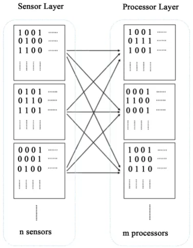
The model consists of a sensor-matrix layer and a processor-matrices layer, each of which contains a certain number of sensor-matrices and processor-matrices respectively. The reason why we can work within two-dimension matrix is that the exact positions of neuron cells are not so important, since essentially speaking, mem-ory depends on not the neurons themselves, but the connections between them. Moreover, due to the complexity of the real process in the human brain which could be far beyond our imagination, not even within three dimen-sions could it be fully illustrated [10]-[12].

Sensors are used to generate perception which responds to a stimulation from the outside world. For instance, our eyes, as a visual sensor, can sense the visual features of the stimulation; ears can sense vocal information and hands can sense tactual information. All the information will then be processed and transmitted to the pro-cessors, where memory-making process takes place (hippocampus) [13]. After the processors received the in-formation from the sensors, the different sorts of inin-formation will be associated together in some ways and forms an initial acquisition of the memory subject. The whole memory process involves three steps, Encoding, Consolidation and Storage, and Retrieval [14] [15]. The transition process from sensors to processors is called encoding step. The association of all sorts of information that the processors received from sensors is regarded as the step for consolidation and storage. For instance, if the visual features of an apple and the literal informa-tion of an apple are associated in a memory process, then next time, one could recall the name, apple, as soon as he or she see an apple. The recalling is viewed related to the retrieval step.

Although this model does not require a particular memory representation, it is useful to illustrate the realiza-tion of all the three steps with a simplified representarealiza-tion.

2.1. Encoding

To simulate transition process, the system with sensors and processors is considered. Each state of the sensors or processors can be stored in a matrix, where each entry represents the state of each neuron cell. The state of a neuron cell is assumed to be either excitatory or inhibitory, which is indicated by binary numbers, that is, 1 and 0, respectively. An example of the encoding process from the sensors to the processors is illustrated inFigure 1.

(3)

Figure 1. Into m correspondence: an excitatory cell is denoted by the number 1.

2.2. Consolidation and Storage

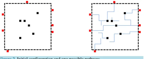
Now constrain our attention to one of the sensors and its corresponding processor, say visual sensor and its cor-responding processor, and the correspondence between them is assumed to be one-to-one. Therefore, the visual processor, which has a spatial structure in the brain, could be simply represented by another n by n matrix. Be-cause the message delivered fast in human brain, the all duration of the transmission from first cell to another cell are regarded equally [17]. At first, the processor received an initial state of excitation from the sensor. Then, the excitation transmission process starts. (It is assumed that the excitation could only conduct from one cell to another once in one stage of the process and it could only be conducted from the newly excited cells. In another word, the cells that have successfully conducted excitation will not be able to conduct excitation any more. After the transmission from first cell to another, a new state of this matrix will be generated). Before the conduction of excitation, the path which used to transmit the excitation between a pair of cell is generated firstly. When the conduction process is finished, the path will be remained there, which forms the memory. The term bridge is used to indicate whether there is path from one cell to another, and noticed that every bridge is represented by a directed line segment. If there is a bridge from cell A to cell B, then it means excitation can be conducted from cell A to cell B. A pair of cells could have at most two bridges between them, opposite in direction. For an illu-stration, the cues of the n by n processor matrix are assumed to lie on the four edges excluding the points at the corners, as is shown inFigure 2. The inner matrix represents the processor with some initial state and the red cells on the peripheral edges around this matrix represent the cues.

The conduction process in a processor is regarded as finished once all the cues received the excitation trans-mitted by bridge and series of excitation cell. The transmission of the excitation is under some conduction rules with neurological significance and it is obvious that the pathway of the excitation will be governed by the cues. Once the initial configuration and the cues are determined, the excitation will be under conduction between cells in the processor and ends up with its reach to the cues. One possible pathway is also shown in Figure 2 where the bridges are indicated by the blue line segments; red cells represent cues.

2.3. Conduction Rules

[image:3.595.219.408.85.327.2]

(4)

[image:4.595.169.460.86.206.2]

Figure 2. Initial configuration and one possible pathway.

can build up bridges to its four adjacent cells, with directions left, right, up and down respectively. The circums-tance with more connections will be considered in later analysis. Thirdly, the transmission process is assumed to be inherently probabilistic. The distance to a cue determines the probability whether the bridge will be estab-lished between the cell and the next cell which is nearer to that cue.

Let O and I denote the sets of cues and original excited cell respectively. Suppose that there are totally m cues and n original excited cells. That is to say, O=O O O1, 2, 3,,Om and I=I I I1, 2, 3,,In. Then theoretically,

the conditional

(

)

3 |

i

O I i j

f = prob O I is determined by

i j i j

k j

O I O I

O I k O

P f

P

∈

=

∑

(1) where P denotes prob O

(

rIt

)

, the probability that events Or and It happen simultaneously. Obviously,

by assumption, the instantaneous set of unreached cues governs the conduction of the next moment. Moreover, the cues could have accumulative effects on the probability of the bridge establishment. After the transmission process, the bridges are kept and stored in the processor, which is regarded as memory.

In the second time, when the figure of apple irritates the sensor again, the excitement will be transmitted au-tomatically through the path established in the first time and all cues will be irritated again which indicates the name, apple.

2.4. Illustration

The model is aimed to simulate the memory process and explore the memory capacity. In another word, it is aimed to find out the limit beyond which the brain would be overloaded and the association of different types of information could be unreachable. For better illustrate, the model is now applied to a specific example with a 30*30 processor matrix. The initial configuration is initialized as shown inFigure 3.

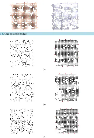
The black dots inside represents the initial state of the processor, which could be an image of an apple. If the red dots outermost refer to the name, apple, then after application of the model, bridges will be established through which the excitation will be conducted until the reach of excitation to all the cues eventually. One poss-ible bridge is shown in Figure 4.

After that, the bridges will be kept as a memory which associates the vision of the apple and its name. Then next time, if the processor receives the information of the apple again, the excitation will be transmitted along the bridges stored automatically and finally reach the cues which indicates the name of the apple. If the proces-sor receives a different piece of information, the excitation will still be transmitted but may not be associated with the same cues, the name apple. For instance, if an image and its name (cues represented by red cells) are defined as shown inFigure 5(a), another different image is indicated in Figure 5(b) input in a short time. Then the name output inFigure 5(a)is different from it in Figure 5(b), so this is a successful case. However in Fig-ure 5(c), another different image obtained by processor in a short time, the name output is totally the same as it inFigure 5(a), which means the images are not be distinguished. Therefore this is a chaotic case [18].

3. Results and Analysis

(5)

[image:5.595.268.363.87.201.2] [image:5.595.169.475.232.682.2]

Figure 3. Initial configuration with black dots indicating the cells in the processor and red dots indicating the cues.

Figure 4. One possible bridge.

(a)

(b)

(c)

(6)

change the percentage of the number of cell with the value of 1 among total number of cells both in image ma-trix and cue layer from 1% to 90%. Then, repeat each test 20 times for each percentage and record the similarity of each different test. The similarity (S) of the results can be calculated by:

1 0 if , 100% 1 if t t n a b t ij G i j G S

i j n

=

≠ 

= ₌ = ×



∑

₍₂₎

where n is the total number of bits in cue layer; at and bt represent the th

t bit in the test sample and the original sample, respectively.

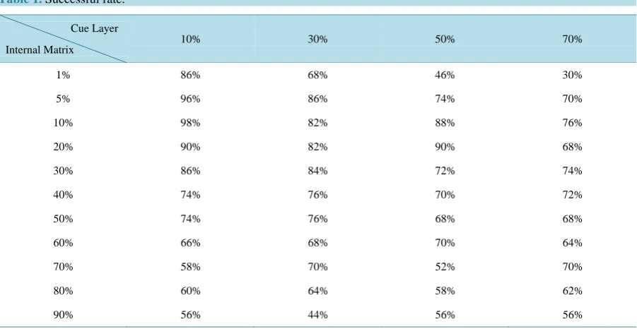
When S equals 1, which means the model cannot tell the difference between the two different images, which is called chaotic. If G is 0, that means the two relative cues are not exactly the same, the difference of the two different images is told by the model. In order to find an optimal condition to distinguish the different image in-formation, first of all, assume that the number of cells with value of 1 in image matrix represents the amount of information stored in the image matrix. The relationship between the whether the processor is chaotic and the number of cells is investigated by using the following method. Adjust the percentage of the cells storing infor-mation and located in image matrix and cue layer from 1% to 90%. Repeat 50 times in every percentage and record the times where the similarity is not equal to 1. Then calculate the successful rate under each condition, where the successful rate is the percentage of the experiment with S = 1 in the whole 50 times experiment. Therefore,Table 1shows the results.

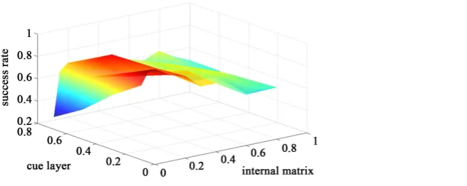
Based onTable 1, a fitting surface is plotted to find the optimal condition, shown inFigure 6.

[image:6.595.88.539.489.722.2]

The top point of the curve in Figure 6with the highest success rate (98%) is the highest point in the whole figure. The condition where the percentage of cells storing information in cue-layer is 10% and the one in image matrix is also 10% is the optimal condition. Therefore, the test result is record which is in condition 10% density image matrix and 10% cue fulfillment. That means when the 10% of the brain space is used to store information, the effect of remembering association is best. That is why in human beings brain, 10% of the storing space is

Table 1. Successful rate.

Cue Layer

Internal Matrix 10% 30% 50% 70%

1% 86% 68% 46% 30%

5% 96% 86% 74% 70%

10% 98% 82% 88% 76%

20% 90% 82% 90% 68%

30% 86% 84% 72% 74%

40% 74% 76% 70% 72%

50% 74% 76% 68% 68%

60% 66% 68% 70% 64%

70% 58% 70% 52% 70%

80% 60% 64% 58% 62%

(7)

[image:7.595.201.529.84.215.2]

Figure 6. Fitting surface of successful rate.

occupied. However, other cells which not hold information are not useless and they are used to transfer excita-tion. In the course of human evolution, the people with a poor memory function are eliminated and the people with brain in the optimal condition are reserved.

Image what would happen if much more storage space is used or unbalanced storage space is used. If 70% of storage space is used both of character part and image part, the successful rate only 70%. That means if you told the patients that image represent an apple, in the next time he may call the other totally different image an apple [20]. Therefore the patients will be diagnosed for a psychopath whose memory is overloaded.

Moreover, in another condition where the two percentages of storage space of character part and image part are different, the function of brain is also influenced. For instance when the character capacity is 10% and the image part is 70%, the success rate is only 58%. That means if the man who has great talent in memorizing im-ages but his capacity of character memorizing is not balanced with it of image memorizing, the man is also has a tendency to be insane. In other words, the genius who has gift on one aspect is nearly lunatic.

Generally, this model can be regarded as a mini-brain. The ability of study depends on the number of cells in use, which means that the length of the period for study decreases with the size of the matrix [21]. The biggest differences between this model and the real brain are the number of cells and the number of connections. There-fore, in this section, matrices with different dimensions and different numbers of connections are adjusted and then the results with different parameters are compared.

Firstly, the dimension of the matrix is expanded to 50 × 50, 80 × 80 and 100 × 100, respectively. Thus, cor-respondingly, the number of neural cells involved increases to 2500, 6400 and 10000, respectively. The condi-tion with 10% density image matrix and 10% cue fulfillment (the optimal condicondi-tion) are set to examine the ef-fect of the size of the matrix on the successful rate. After that the case with dimension 50 × 50 has been repeated 50 times and a new successful rate 98% was obtained which is also comparatively high. The cases with dimen-sion 80×80 and 100 × 100 were tested and the successful rates are 100% and 98%, respectively. Therefore, we can speculate that the successful rate may be independent from the size of matrix.

Secondly, in order to investigate whether the number of connections can affect the results of the experiment, we double the number of connections and observe, i.e., not only the up, below, left and right adjacent cell are connected to the central cell but also the up-right, up-left, bottom-left and bottom-right adjacent cell can be as-sociated. Two pieces of different image information are given under the optimal condition. The relative cue- layers are different so the two pieces of image are successfully distinguished.

After that, the experiment has been repeated 50 times and the successful rate obtained is 100%. Therefore we can speculate that the number of connections may not influence the successful rate either.

According to the statistics, the dimension and the number of connections may have no effect on the successful rate. Therefore, we can conclude that the percentage of optimal occupied space in the brain is about 10%.

Finally, to simplify the computation and programming, the number of connections that a neuron cell could have with the adjacent cells is up to eight in this model. However, in fact, thousands of connections could be made by one single cell [21].

Hence, further study could enlarge the matrix. Since in the model the matrix used to represent the processor has comparatively small dimensions, the processor is considered as a whole. When the matrix becomes larger and larger, partition of the processor could be taken into consideration.

(8)

ther than unexploited. Furthermore, it can be speculated that the successful rate may be independent from the size of the matrix. And the dimension and number of connections may have no effect on the successful either.

Acknowledgements

This work was supported by grants from the National Natural Science Foundation of China (No.11204245), and the Natural Science Foundation of Jiangsu Province (No. BK2012637).

References

[1] Grossi, E. and Buscema, M. (2007) Introduction to Artificial Neural Networks. European Journal of Gastroenterology

and Hepatology, 19, 1046-1054. http://dx.doi.org/10.1097/MEG.0b013e3282f198a0

[2] Mastin, L. (2015) Long Term Memory. http://www.human-memory.net/types\_long.html

[3] Ma, C. and Zhang, N. (2015) Transforming Growth Factor Beta Signaling Is Constantly Shaping Memory T-Cell

Pop-ulation. Proceedings of the National Academy of Sciences of the United States of America, 112, 11013-11017.

http://dx.doi.org/10.1073/pnas.1510119112

[4] Vogels, T.P., Sprekeler, H., Zenke, F., Clopath, C. and Gerstner, W. (2011) Inhibitory Plasticity Balances Excitation

and Inhibition in Sensory Pathways and Memory Networks. Science, 16, 1569-1573.

http://dx.doi.org/10.1126/science.1211095

[5] Hartmann, K., Bruehl, C., Golovko, T. and Draguhn, A. (2008) Fast Homeostatic Plasticity of Inhibition via Activity-

Dependent Vesicularlling. PLoS ONE,3, e2979. http://dx.doi.org/10.1371/journal.pone.0002979

[6] Huxley, A.F. (1964) Excitation and Conduction in Nerve: Quantitative Analysis. Science, 145, 1154-1159.

http://dx.doi.org/10.1126/science.145.3637.1154

[7] Okun, M. and Lampl, I. (2008) Instantaneous Correlation of Excitation and Inhibition during Ongoing and Sensory-

Evoked Activities. Nature Neuroscience, 11, 535-537. http://dx.doi.org/10.1038/nn.2105

[8] Luksys, G., et al. (2015) Computational Dissection of Human Episodic Memory Reveals Mental Process-Specific

Ge-netic Profiles. Proceedings of the National Academy of Sciences of the United States of America, 112, 4939-4948.

[9] Kawato, M. and Gomi, H. (1992) The Cerebellum and VOR/OKR Learning Models. Trends in Neurosciences, 15, 445-

453. http://dx.doi.org/10.1016/0166-2236(92)90008-v

[10] Machens, C.K., Romo, R. and Brody, C.D. (2005) Flexible Control of Mutual Inhibition: Aneural Model of Two-In-

terval Discrimination. Science, 307, 1121-1124. http://dx.doi.org/10.1126/science.1104171

[11] Nenert, R., Allendorfer, J.B. and Szaarski, J.P. (2014) A Model for Visual Memory Encoding. PLoS ONE,9, e107761.

http://dx.doi.org/10.1371/journal.pone.0107761

[12] Flores, C.E., et al. (2015) Activity-Dependent Inhibitory Synapse Remodeling through Gephyrin Phosphorylation.

Proceedings of the National Academy of Sciences of the United States of America, 112, E65-E72.

[13] Nielsona, D.M., Smitha, T.A., Sreekumara, V., Dennisa, S. and Sederberga, P.B. (2015) Human Hippocampus Repre-

sents Space and Time during Retrieval of Real-World Memories. Proceedings of the National Academy of Sciences of

the United States of America, 112, 11078-11083. http://dx.doi.org/10.1073/pnas.1507104112

[14] Mastin, L. (2010) The Human Memory. http://www.human-memory.net/types_short.html.

[15] Nomura, H., et al. (2015) Memory Formation and Retrieval of Neuronal Silencing in the Auditory Cortex. Proceedings

of the National Academy of Sciences of the United States of America, 112, 9740-9744.

[16] Markowitza, D.A., Curtisa, C.E. and Pesarana, B. (2015) Multiple Component Networks Support Working Memory in

(9)

11089. http://dx.doi.org/10.1073/pnas.1504172112

[17] Wada, N., Funabiki, K. and Nakanishi, S. (2014) Role of Granule-Cell Transmission in Memory Trace of Cerebellum-

Dependent Optokinetic Motor Learning. Proceedings of the National Academy of Sciences of the United States of

America, 111, 5373-5378. http://dx.doi.org/10.1073/pnas.1402546111

[18] Vreeswijk, C.V. and Sompolinsky, H. (1996) Chaos in Neuronal Networks with Balanced Excitatory and Inhibitory

Activity. Science, 274, 1724-1726. http://dx.doi.org/10.1126/science.274.5293.1724

[19] McTighe, S.M., Cowell, R.A., Winters, B.D., Bussey, T.J. and Saksida, L.M. (2010) Paradoxical False Memory for

Objects after Brain Damage. Science, 330, 1408-1410. http://dx.doi.org/10.1126/science.1194780

[20] Yger, P., Stimberg, M. and Brette, R. (2015) Fast Earning with Weak Synaptic Plasticity. The Journal of Neuroscience,

35, 13351-13362. http://dx.doi.org/10.1523/JNEUROSCI.0607-15.2015

[21] Gerstner, W. and Naud, R. (2009) How Good Are Neuron Models. Science, 326, 379-380.