2645
EXPLORING THE DENSITY-DEPENDENT STRUCTURE OF BLOWFLY
POPULATIONS BY NONPARAMETRIC ADDITIVE MODELING
OLE C. LINGJÆRDE,1NILSCHR. STENSETH,1,4ANJAB. KRISTOFFERSEN,1ROBERTH. SMITH,2S. JANNICKE MOE,1 JONATHANM. READ,2SUSANDANIELS,3ANDKENSIMKISS3
1Department of Biology, University of Oslo, P.O. Box 1050, N-0316 Oslo, Norway 2Department of Biology, University of Leicester, University Road, Leicester LE1 7RH UK
3School of Animal Microbial Sciences, University of Reading, Reading RG6 2AJ UK
Abstract. Abundances of 12 laboratory populations of the greenbottle blowfly (Lucilia
sericata) were recorded every two days for 776 d, with separate counts for larvae, pupae,
and adults. Half of the populations were exposed to sublethal dosages of the toxic compound cadmium acetate; the remaining populations were considered controls. Initial density was low for half of the populations in each group, and high for the other half. In all populations, the adult abundance underwent sustained fluctuations. However, cadmium-exposed popu-lations had smaller mean larval and adult densities, and fluctuations in adult abundance were less regular than for controls. Data from the first and the second half of the experimental period were analyzed separately in order to assess the effects of possible long-term changes in the dynamics on the estimates. Nonparametric (generalized) additive modeling (GAM) was used to investigate time series dynamics and, in particular, to explore the density-independent components and the structure of the density-dependent components of the system. Overall, cadmium populations had larger larva-to-adult survival rate and smaller adult survival rate than control populations, and for the second half of the experimental period the reproductive rate was smaller for cadmium populations than for control popu-lations. Estimation of the density-dependent components suggested that survival from larva to adult depended nonlinearly on larval density and that increased larval density had a positive effect on larval survival at low densities. Furthermore, cadmium generally de-creased vital rates. However, the analysis suggested that most of the observed differences in dynamical behavior between control and cadmium populations are related to differences in the density-independent components of the demographic rates, rather than differences in the density-dependent structure.
Key words: additive models; greenbottle blowfly; cadmium; density-dependent and density-in-dependent components; ecotoxicology; generalized additive model (GAM); Lucilia sericata; nonli-nearities; nonparametric regression; population model; time series analysis.
INTRODUCTION
Nicholson’s (1954a, 1957) work on the population
dynamics of the sheep blowflyLucilia cuprina has held
a major position in the development of the field of population ecology (Gurney et al. 1980, Begon et al. 1996). Nicholson emphasized the role of population-intrinsic density-dependent factors in determining pop-ulation dynamic behavior, and his classic laboratory experiments, reported in Nicholson (1954a, b), were
designed to demonstrate what he regarded as a ‘‘self-evident truth’’ (J. L. Readshaw, personal communi-cation). His view has often been contrasted with that
of Andrewartha and Birch (1954), who focused on the role of population-extrinsic (generally abiotic) density-independent factors in determining population dynamic behavior. Today there is general agreement that both density-dependent and density-independent factors are important for understanding the overall dynamics of a
Manuscript received 24 June 1999; revised 27 March 2000; accepted 10 April 2000; final version received 3 October 2000.
4Corresponding author. E-mail: [email protected]
population (Turchin 1995, Leirs et al. 1997). Earlier interpretations of population data largely equated in-trinsic population control with stability, and exin-trinsic, abiotic control with instability and large fluctuations. However, it should never be forgotten that some sort of density dependence is needed for maintaining any population (Orzack 1997). Focusing on the density-dependent structure, May (1976) demonstrated in his pioneering paper that nonlinear density dependencies may give rise to very complicated dynamical behavior in rather simple population models.
2646 OLE C. LINGJÆRDE ET AL. Ecology, Vol. 82, No. 9
FIG. 1. Demographic rates with identical density-depen-dent components (nonlinear in this case) and different den-sity-independent components.
Daniels (1994) reported on a replicated 2 32 fac-torial experiment with blowfly populations (Nichol-son’s [1954a, b] experiments were not replicated), with
larval competition as the main density-dependent fac-tor. Experimental factors were exposure to the toxic heavy metal cadmium (no exposure or a sublethal dose) and initial population density (low or high). Our main interest is in determining whether exposure to cadmium affects vital rates; the initial density factor may be con-sidered a ‘‘blocking’’ variable introduced to increase the sensitivity of the inference for cadmium treatment. Cadmium, an abiotic density-independent factor, is one of the most toxic nonessential elements found in the environment. The main toxic effect is its ability to dis-place copper and zinc ions from their binding sites in metalloproteins, which destroys the biological prop-erties of many enzymes. Cadmium may also substitute calcium in several physiological processes. Earlier analyses and modeling approaches using these data have been reported by Smith et al. (2000). Here, we report further on the empirical modeling of these pop-ulation data.
Various statistical approaches have been used to an-alyze (relatively short) ecological time series, including computer-intensive methods such as nonlinear fore-casting and response surface methodology (Sugihara and May 1990, Ellner and Turchin 1995, K.-S. Chan, H. Tong, and N. C. Stenseth,unpublished manuscript).
Statistical modeling approaches may broadly be divid-ed into parametric and nonparametric methods (Bow-man and Azzalini 1997); the choice between these de-pends on the purpose of the analysis, as well as on the amount of data available. For answering specific ques-tions about well-defined ecological quantities, para-metric models have the benefits of easy interpretation and a well-developed inferential theory. At the first stage of an analysis there may, however, be more em-phasis on establishing general features of the dynamical system, like the presence and shape of nonlinearities in the density-dependent structure. In this part of the study, nonparametric models are potentially very use-ful. Making minimal assumptions about the functional forms, such models allow the data to ‘‘speak for them-selves’’. Furthermore, nonparametric methods can be used to test the adequacy of parametric models (Hart 1997). In general, nonparametric estimators may be expected to have small bias and usually a lower order of convergence than their parametric counterparts, hence for small data sets a well-chosen parametric es-timator will usually outperform nonparametric esti-mators in terms of mean square error (Hart 1997). How-ever, it is often difficult to know what an appropriate parametric model would be for a given problem, and nonparametric models may therefore be useful even in situations involving small amounts of data. Here we use a particular class of nonparametric models known as generalized additive models (GAM; e.g., Hastie and Tibshirani 1990; for ecological applications of such
models, see, e.g., Stenseth et al. [1997], Bjørnstad et al. [1998]).
As an interpretive aid, it is commonly useful to con-sider population dynamical behavior as an interaction between a deterministic and a stochastic component (Stenseth et al. 1998). The relative importance of these components is closely related to the issue of density-dependent vs. density-indensity-dependent control. Typically, within the field of statistical modeling of ecological time series data (Stenseth et al. 1997, Bjørnstad et al. 1998), the skeleton (sensu Tong 1990) represents the deter-ministic component. The stochastic component is often further divided into (cf. May 1973) demographic sto-chasticity (typically related to the density-dependent components of the model) and environmental stochas-ticity (typically related to the density-independent com-ponents of the model). In general, the observed popu-lation dynamical behavior may be the result of a com-plex interaction between the deterministic and the stochastic components (Takens 1994, Tong 1995, Wie-senfeld and Moss 1995). For example, in a nonlinear deterministic system generating limit cycles, introducing stochasticity may alter the dominant period of the at-tractor (Stenseth et al. 1998). As a consequence, one should distinguish between studies aimed at understand-ing general structural features of the system and the more ambitious task of building a realistic model capturing all observed population dynamic features. Here we re-strict ourselves to the former.
difference between these two components. The func-tional shape of the latter component (e.g., whether it is nonlinear) will be a main target in the analysis we present. A secondary aim is to discover whether ex-posure to a density-independent factor (cadmium) has any effect on the demographic rates. Since cadmium may affect development and survival, increased larval mortality may be experienced at high larval densities, introducing an interacting effect between a density-independent factor and a density-dependent factor.
THEDATA
Our data represent observations on the temporal fluc-tuations in 12 laboratory populations of the greenbottle blowfly Lucilia sericata Meigen, the northern
hemi-sphere sister species of L. cuprina, over a period of
776 d. These experiments, carried out at the University of Reading during 1989–1992, are described in detail by Daniels (1994) and Smith et al. (2000). Colonies were kept in separate plastic tanks at 258C and 60% relative humidity on a 12 h/12 h light/dark regime. The diet, provided both in fresh and dried form, consisted of 20 g/kg agar containing 20% (by volume) horse blood and 50 g/kg dried brewers yeast (20 g fresh diet per population, fully replaced every two days). The fresh diet served both as a medium for oviposition and as food, primarily for the larvae and to some extent also for the adults. Larvae were allowed to migrate into vermiculite surrounding the diet pot for pupating. Su-crose, water and dried diet were provided ad libitum for adults.
The blowfly populations were divided into four ex-perimental groups, each consisting of three replicates. Cadmium acetate was given through fresh and dried diet (50 mg cadmium/kg fresh diet) to six treatment populations; the remaining six populations were con-sidered controls. The three populations in each low-density group were initiated with 30 pupae and 30 adults, whereas the three populations in each high-den-sity group were initiated with 150 pupae and 150 adults. In the following, we refer to the populations by the termscontrol (CON), cadmium (CAD), each
subdivid-ed into low density (L) and high density (H): for
ex-ample, CON(L) refers to all three low-density control populations, whereas CAD(H3) refers to the third high-density cadmium treatment population.
The data consist of a panel with 3312 time series, giving counts every two days for three different life stages in each population: larva, pupa, and adult (eggs were not counted). All time series span the same period and were collected by the same personnel. Counts of premigratory larvae and adults include all age groups, whereas pupal counts only include those pupating dur-ing the last two days (i.e., since the last count). Only
viable pupae (i.e., pupae surviving long enough to
be-come adults) are included in the counts used here (Smith et al. [2000] included both viable and nonviable pupae in their analyses).
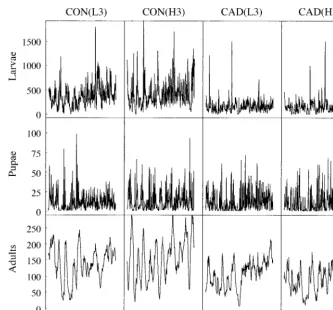
Time series data for larvae, pupae, and adults are shown in Figs. 2–4. A qualitative change is seen in some features when comparing control populations (the first two columns of Figs. 2–4) with cadmium popu-lations (the last two columns of Figs. 2–4). Notice that one cadmium population (CAD[L2]) went extinct be-fore the end of the experiment; this population is ex-cluded from our analyses.
In the analyses, combining data from all replicates proved useful, since it led to substantial reduction in the variance of the estimators. However, to evaluate the degree of consistency among the replicates, they were also analyzed separately.
MODELINGSTAGE-STRUCTUREDINTERACTIONS
Stochastic state transition models (Ebenman and Pearsson 1988) are frequently used to describe tem-poral population fluctuations (Caswell 1989a, b).
As-sume for this purpose that the life cycle of the species under consideration is divided into d age classes of
equal duration; letNt,1,. . . ,Nt,ddenote the population
abundances for each age class at time t.
The model describing the population-dynamic pro-cess relates the state of the system at timet11, defined as Nt115 (Nt11,1, . . . ,Nt11,d)T, to earlier states. Anal-ogous to a Leslie matrix representation, this may be expressed as
Nt11 5A(N , Nt t21,. . . ,Nt2q;nt)N .t (1)
The transition matrix A(Nt, Nt21, . . . , Nt2q; nt) may
depend on the state of the system at previous time steps (t, t 2 1, . . . ,t2 q) as well as on a stochastic term
nt. For a given population system, the appropriate form
of Eq. 1 will depend on the chosen time unit. Based on the approximation that there are four life stages (larva, pupa, immature adult, and mature adult) each lasting eight days, Smith et al. (2000) use a time step of eight days in their statistical modeling of the same data. Considering the differences in the actual time span of each life stage (see Table 1), a model based on a smaller time step than eight days may be able to capture the dynamics of the system more accurately. Here, we use a time step of two days (i.e., equal to the frequency of observation).
2648 OLE C. LINGJÆRDE ET AL. Ecology, Vol. 82, No. 9
FIG. 2. Stage-specific abundances of four L. sericata populations, counted every two days over a period of 776 d.
Abbreviations are: CON, control; CAD, cadmium; L, low density; H, high density; ‘‘1’’ denotes first replicate.
the model, at the expense of making the model more detailed and possibly more complicated. We adopted the latter approach, since it requires only the recorded variables for estimation.
The model to be described consists of a number of equations of the form
Nt11,k5Nt,k0exp[a 1 g (log N1 t2t,k1)1g (log N2 t2t,k2)]
(2)
whereNt,kdenotes thekth element of the state vector Nt,
t$0 is a time delay,ais a constant, andg1andg2are smooth functions (see the Appendix for a technical def-inition of smooth functions), one or both of which may be absent. The variablesNt,k0andNt11,kcorrespond to sub-sequent age groups in the blowfly life cycle; thus the exponential factor in Eq. 2 represents either rate of sur-vival or rate of reproduction, depending on the context. The per-unit-abundance net growth rate is defined as log
Nt11,k2logNt,k0and is assumed to be an additive function
oflogNt2t,k1and logNt2t,k2 plus noise. Density indepen-dence (respectively density depenindepen-dence) corresponds to havingg1[g2[0 (respectivelyg1±0 for at least one function). In the case of density independence, the per-unit-abundance rate is simply a constant. In the case of density dependence, the per-unit-abundance rate
decreas-es (respectively increases) as a function of , 0 (respectively .
Nt2t,kiwhengi9(Nt2t,ki) gi9(logNt2t,ki)
0), where the prime indicates differentiation.
STAGESTRUCTUREREPRESENTATION
Model assumptions
For modeling purposes, we make the assumption that the blowfly life history consists of four basic devel-opmental stages:egg/larva, pupa, immature adult and mature adult. Approximate length of each stage is
shown in Table 1; some stages have a length that de-pends on the treatment. Here, we assume that the larval stage lasts for eight days, the pupal stage lasts for 10 d, and the immature adult stage lasts for four days. As a consequence, stage durations are assumed to be den-sity independent. The life span of mature adults has no specified upper limit. A separate egg stage has not been included in the model, in part because data are not available on the number of eggs. Since hatching is com-pleted within roughly one day (Daniels 1994), omitting this stage from the model is not in conflict with a time step of two days. A further modeling assumption is that the demographic rates are identical for all individuals within a given age group.
FIG. 3. Stage-specific abundances of fourL. sericata populations, counted every two days over a period of 776 d. The
population CAD(L2) went extinct after 298 d. See Fig. 2 legend for definitions; ‘‘2’’ denotes second replicate.
to have identical density-dependent structure. The re-productive rate is assumed to depend only on the den-sity of mature adults. Assuming that any effects of density on the larvae manifest themselves on survival in the transition from larva to (viable) pupa, the sur-vival probability of a larva from one age group to the next will be density independent. The proportion of larvae pupating (to viable pupae) at any given time is modeled as a function of the total number of larvae
four days before. The latter quantity serves as a proxy (up to a proportionality factor) for the number of larvae in the feeding phase at the time the currently pupating larvae were feeding. This reflects the expectation that density-dependent effects to be found in the larval stage are related to the feeding conditions of the larvae.
Note that, since pupal counts include only theviable pupae, the only way to leave the pupal stage is to
become an adult. Since the immature stage accounts for only a small part of the whole adult stage (;5 out of 17 d), we make the assumption that no deaths occur in the immature adult stage (this greatly simplifies the estimation process). As long as we do not ask for the death rate amongst immature and mature adults sepa-rately, but only theoverall death rate within the adult
stage, little harm is done by making this assumption.
The model
A stage-structured model for the population dynam-ics will now be presented. Let
i
Lt[population of larvaed∈[2i22, 2i ] days old
at timet
i
Pt [population of pupaed∈[2i22, 2i ] days old
at timet
i
At[population of adultsd∈[2i22, 2i ] days old
at timet
where the range of the superscript i ∈{1,. . . , 4} in the first definition, {1,. . . , 5} in the second, and {1,2,3,. . . } in the third. Superscripts indicate age groups within a stage (i.e., members differing at most two days in age within a stage). Abundances of im-mature adults and im-mature adults at time t are
approx-imated by
2
I j
At5
O
At (immature adults at timet)j51
`
M j
At 5
O
At (mature adults at timet). (3)2650 OLE C. LINGJÆRDE ET AL. Ecology, Vol. 82, No. 9
FIG. 4. Stage-specific abundances of fourL. sericata populations, counted every two days over a period of 776 d. See
Fig. 2 legend for definitions; ‘‘3’’ denotes third replicate.
TABLE1. Approximate time span (in days) of each stage in the life cycle ofL. sericata.
Life stage
Control populations
Cadmium populations Egg and larva
Pupa
Immature adult Mature adult
8 6–12
5 12
9 6–12
5 9
Note: Some of the numbers in the table depend on larval
density, as well as on other factors.
Furthermore, note that the total size of the larval pop-ulation at timet is
4
j
Lt5
O
L .t (4)j51
The stage-structured model is given by the following set of equations:
1 M M
Lt115A exp[t a 1L1 f (log A )]L t (5)
i11 i
Lt115L exp(t aL2) 1#i# 3 (6)
1 4
Pt115L exp[t a 1P f (log LP t21)] (7)
i11 i
Pt11 5Pt 1#i#4 (8)
2 1 5
At115At 5Pt21 (9)
i11 i I M
At115A exp[t a 1A f (log A )A1 t 1 f (log A )]A2 t
2#i, ` (10)
where the smooth functions (fL,fP,fA1, andfA2) and the parameters (aL1,aL2,aP, andaA) correspond to the den-sity-dependent and density-independent components of the demographic rates, respectively. When no confu-sion can arise, we refer to the parameter values simply as reproduction rate, larval survival rate, and so on.
The particular form of the model in Eqs. 5–10 is similar to, e.g., the larva–pupa–adult (LPA) model (Dennis et al. 1995). However, the latter model is based on only three stages and assumes linear functions inside the exponentials rather than general smooth functions.
Statistical methods
[image:6.612.134.468.90.400.2] [image:6.612.307.523.649.711.2]den-FIG. 5. Nonparametric trend estimates for all the time series, considered as functions of the observation times. Each curve was found by smoothing one of the time series with a cubic smoothing spline using seven degrees of freedom.
sity-dependent components (functions); see the Ap-pendix for more details about the estimation procedure. To compare parameter values, simple parametric tests such as thet test are not applicable, due to the
unknown distributional properties of the parameter es-timates. Instead, we resort to using two nonparametric tests, one for testing whether two samples could have come from populations with the same mean (the Mann-Whitney [MW] U test), and one for testing whether
two samples could have come from identical distri-butions (the Kolmogorov-Smirnov [KS] test). Both tests assume that the samples are mutually independent random samples; since samples correspond to inde-pendent populations (trials), this is a reasonable as-sumption. Formal statistical comparison of function shapes is a difficult problem and will not be treated here (but see Bowman and Azzalini [1997] for a dis-cussion of this topic for models involving a single smooth function). Rather, we emphasize the explorato-ry nature of our analysis and simply compare function shapes visually.
All the time series analyzed as part of this study have long-term trends (Fig. 5), and most show reduced var-iability in pupal and adult counts towards the end of the experimental period (Fig. 6). The long-term trends consist of an initial decline phase lasting for ;200– 300 d (depending on which life stage we consider),
followed by an increase phase lasting an additional 200–300 d. The trends then appear to level off. To examine the effects of the long-term trends on the es-timated rates, each time series was split into two halves of equal length, denoted part I and part II, which were analyzed separately.
The model in Eqs. 5–10 was first estimated for four different sets of data, each being the result of combin-ing data from all three replicates of CON(L), CON(H), CAD(L), or CAD(H). As a check of consistency be-tween replicates, we also estimated the model for in-dividual replicates. We found that estimates derived from data on single replicates are very similar. Fur-thermore, the effect on the estimates of initial popu-lation density seems negligible.
RESULTS
Density-independent components of demographic rates
2652 OLE C. LINGJÆRDE ET AL. Ecology, Vol. 82, No. 9
FIG. 6. Nonparametric standard-error estimates for all the time series. Each curve was found by smoothing one of the time series (considered as a function of the observation times), then smoothing the time series of squared residuals from the first smooth, and finally taking the square root. Smooths were computed using a cubic smoothing spline with five degrees of freedom.
Cadmium populations have significantly larger lar-va-to-adult survival rate (aP) and smaller adult survival rate (aA) than control populations (pMW,0.01 andpKS ,0.01 in both cases, both for part I and part II). Cad-mium populations have significantly smaller reproduc-tive rate than control populations in part II (pMW50.03 andpKS50.03), but not in part I.
Reproductive rate (aL1) increases significantly from part I to part II (pMW,0.01 and pKS,0.01, for both control populations and cadmium populations). For control populations, larva-to-adult survival rate (aP) decreases significantly (pMW, 0.01 and pKS 5 0.03) and adult survival rate (aA) increases significantly (pMW , 0.01 and pKS , 0.01) from part I to part II of the experiment. A change of parameters from part I to part II is consistent with the presence of long-term trends.
Density-dependent components of demographic rates
Fig. 8 shows function estimates based on all repli-cates within each of the four experimental groups. Functions are quite similar, even when comparing cad-mium populations and control populations. The larva-to-adult survival curve (fP) is markedly nonlinear, il-lustrating the usefulness of empirical modeling in dis-covering the nature of functional relationships. The
curvefPis increasing for low larval densities and (ex-cept for part I of CAD[H]) decreasing for higher den-sities. On the other hand, there is no apparent effect of adult density (neither immature nor mature) on the adult survival rate (fA1andfA2). The estimated
repro-duction curve (fL) decreases markedly with adult den-sity.
Fig. 9 shows plots of function estimates for each of the eleven populations that persisted. There is again a high degree of consistency between the results obtained for different replicates.
DISCUSSION
TheLucilia sericata data analyzed in this study
high-FIG. 7. Estimate of the density-independent component of the demographic rates, for individual populations (shown as circles) and for the four experimental groups (shown as filled triangles), for the model in Eqs. 5–10. For each parameter in each panel, the left-most three (two in the case of the cadmium treatment) circles correspond to the L (low initial density) replicates, and the right-most three circles correspond to the H (high initial density) replicates. The two filled triangles are pooled estimates for the entire L group and the entire H group, respectively. Note that parameter values are plotted as exp(a) for the various replicates.
TABLE2. Tests for equal location of parameters in control and cadmium populations (testing part I and part II separately) and in part I and part II (testing control and cadmium populations separately), using a two-sided alternative; entries are probability values.
Parameter
Control vs. cadmium Part I
pMW pKS
Part II
pMW pKS
Part I vs. part II CON
pMW pKS
CAD
pMW pKS
aL1 1.00 0.97 0.03 0.03 ,0.01 ,0.01 ,0.01 ,0.01
aL2 0.79 0.90 0.54 0.69 0.24 0.47 0.15 0.36
aP ,0.01 ,0.01 ,0.01 ,0.01 ,0.01 0.03 0.84 0.87
aA ,0.01 0.03 ,0.01 ,0.01 ,0.01 ,0.01 0.10 0.08
Notes: Probability values are given both for a two-sample Mann-Whitney U test (pMW) and for a two-sample
Kolmogorov-Smirnov test (pKS). Abbreviations are: CON, control; CAD, cadmium. lights the obvious value of replication (Smith et al.
2000) in ecological time series studies.
General features of the model
There is no significant effect of adult density on the adult survival rate (fA1andfA2). This result is not sur-prising, considering that adults are fed ad libitum, and consequently adults supposedly have no need to com-pete for food. Nevertheless, the estimated reproduction curve (fL) decreases markedly with adult density.
Pos-sible explanations for this include reduced fecundity due to other kinds of stress experienced by adults at high densities, local mate competition, and the fact that the total reproduction is limited by the area suitable for oviposition (the fresh diet). The negative slope of
fLcould also be a delayed effect of competition at the larval stage, which may reduce body size and therefore fecundity of these individuals as adults (Ullyett 1950, Nicholson 1954a). Such an effect could easily have
appro-2654 OLE C. LINGJÆRDE ET AL. Ecology, Vol. 82, No. 9
FIG. 8. Estimate of the density-dependent component of the demographic rates, for each of the four experimental groups, for the model in Eqs. 5–10. Approximate 95% confidence bands are also shown (dotted lines). Argument values are shown as rug plots along the abscissas. Functions are centered (see the Appendix) and are plotted on the same range. Estimates for CAD(L) are based on data for CAD(L1) and CAD(L3) only.
priate data (requiring additional experiments) we can-not determine whether or can-not this effect is the real cause for the decrease in the estimated reproduction rate.
Larval competition is known to be an important com-ponent of blowfly population dynamics (Nicholson 1950). Based on the observation that reduction in the amount of food per larva leads to reduced growth and survival ofL. sericata, Simkiss et al. (1993) concluded
that increasing larval densities have negative effects
FIG. 9. Estimate of the density-dependent component of the demographic rates, for all 12 populations, for the model in Eqs. 5–10. Functions are centered (see the Appendix) and are plotted on the same range. Estimates for CAD(L2) are not shown.
1987), and may therefore contribute to increased growth and survival of the larvae. Yet, at higher den-sities, competition results.
Effects of cadmium
Although cadmium has a significant effect on some demographic rates (larva-to-adult survival rate [aP] and adult survival rate [aA], and for part II also reproduc-tion rate [aL1]), the effect on the density-dependent components appears (by visual examination) to be
2656 OLE C. LINGJÆRDE ET AL. Ecology, Vol. 82, No. 9
may thus be a result of reduced density-dependent lar-val mortality.
Concluding comments
Nonparametric regression has allowed us to dis-entangle the density-dependent effects, as well as the density-independent effects, at different stages under various environmental conditions (for another ex-ample, see, e.g., Leirs et al. [1997]). Indeed, the non-parametric approach is a very valuable first step in the development of data-based population models. It is by taking such an open-minded view that we are able to detect new (i.e., not previously appreciated) patterns in the way different stages interact. This novel insight provides a basis for more detailed ex-perimental studies (aiming at verifying or rejecting the patterns suggested on the basis of this kind of time series modeling). Analysis that incorporates greater detail of the emerging dynamics will be fur-ther facilitated by having a parameterized model, since we then more easily can study the effect of changing the strength of, e.g., the density-dependent effects.
Further work suggested by these results falls into two categories. On the statistical side, the model could be extended to include interaction terms, the signifi-cance of which should then be tested in the treatment and the control group. The statistical significance of the effect of cadmium on the population dynamics should be tested formally, following formal testing of common structures for panels of time series (Tong 1990, K.-S. Chan, H. Tong, and N. C. Stenseth, un-published manuscript). The current results can then
be used to develop simpler, parametric models that are easier to analyze mathematically (cf. Smith et al. 2000).
On the experimental side, short-term experiments are needed in order to test hypotheses about model struc-ture. In particular, one may investigate the modeling assumption that different age groups within a life stage have identical density-dependent structure. Forrest (1996) investigated the density dependence from larvae to pupae using even-aged cohorts. However, compe-tition between different larval instars is likely to be asymmetric, and future experiments should examine the effects of both larval age structure and density on adult emergence.
Finally, we argue that this sort of experimental and analytical approach can yield new insights into areas of applied ecology such as ecotoxicology. We noted above that flies in cadmium populations overall have lower fecundity than control flies, hence the cad-mium populations do not rise to such high densities and are not as strongly affected by nonlinearities as are the control populations. One consequence of this is that the mean biomass production at the pupal stage is higher for the cadmium than for the control populations (Daniels 1994), even though
conven-tional ecotoxicology dogma would predict the op-posite: the simple prediction would be that individ-uals exposed to a toxin such as cadmium should have less energy available for growth and reproduction (i.e., reduced ‘‘scope for growth’’), hence contrib-uting to a lower average biomass per population. In practice, the interaction of the toxin with the strongly nonlinear density dependence produced an emergent property at the population level that is at variance with the simple scope-for-growth prediction. This highlights the importance of dissecting out the struc-ture of population processes using experimentation and nonparametric regression techniques in order to be able to understand and to predict effects at the population level.
ACKNOWLEDGMENTS
The analysis reported in this paper has mostly been sup-ported by the Norwegian Science Council (NFR): O. C. Lingjærde was supported by a grant to N. C. Stenseth from NFR (the Ecotoxicology Programme). A. B. Kristoffersen was supported by a grant to N. C. Stenseth from NFR (Stra-tegic University Programme). S. J. Moe was supported by a doctoral stipend from NFR. S. Daniels was supported by three successive small grants from the UK Natural Environment Research Council (NERC) to R. H. Smith and K. Simkiss during the period of data collection. J. M. Read is supported by a grant from the NERC to R. H. Smith. We thank Mike Begon, Steve Ellner, and Ottar Bjørnstad for valuable com-ments to earlier versions of this paper. We also thank two anonymous reviewers and the associate editor Edward F. Con-nor for valuable input during the preparation of the final man-uscript.
LITERATURECITED
Andrewartha, H. G., and L. C. Birch. 1954. The distribution and abundance of animals. University of Chicago Press, Chicago, Illinois, USA.
Begon, M., J. L. Harper, and C. R. Townsend. 1996. Ecology: individuals, populations and communities. Third edition. Blackwell Scientific, Oxford, UK.
Begon, M., S. M. Sait, and D. J. Thompson. 1995. Persistence of a parasitoid–host system—refuges and generation cy-cles. Proceedings of the Royal Society of London Series B 260:131–137.
Bjørnstad, O. N., M. Begon, N. C. Stenseth, W. Falck, S. M. Sait, and D. J. Thompson. 1998. Population dynamics of the Indian meal moth: demographic stochasticity and de-layed regulatory mechanisms. Journal of Animal Ecology
67:110–126.
Bowman, A. W., and A. Azzalini. 1997. Applied smoothing techniques for data analysis. The kernel approach with S-Plus illustrations. Clarendon, Oxford, UK.
Caswell, H. 1989a. Matrix population models: constructions,
analysis and interpretation. Sinauer, Sunderland, Massa-chusetts, USA.
Caswell, H. 1989b. Analysis of life table response
experi-ments. 1. Decomposition of effects on population growth rate. Ecological Modelling 46:221–238.
Daniels, S. 1994. Effects of cadmium toxicity on population dynamics of the blowflyLucilia sericata. Dissertation.
Uni-versity of Reading, UK.
Dennis, B., R. A. Desharnais, J. M. Cushing, and R. F. Con-stantino. 1995. Nonlinear demographic dynamics: mathe-matical models, statistical methods, and biological exper-iments. Ecological Monographs 65:261–281.
popu-lations: ecology and evolution. Springer-Verlag, Berlin, Germany.
Ellner, S. P., and P. Turchin. 1995. Chaos in a noisy world: new methods and evidence from time series analysis. Amer-ican Naturalist 145:343–374.
Forrest, 1996. Toxins and blowfly populations. Dissertation. University of Leicester, UK.
Gurney, W. S. C., S. P. Blythe, and R. M. Nisbet. 1980. Nicholson’s blowflies revisited. Nature 287:17–21. Gurney, W. S. C., S. P. Blythe, and T. K. Stokes. 1999. Delays,
demography and cycles: a forensic study. Advances in eco-logical research 28:127–144.
Gurney, W. S. C., and R. M. Nisbet. 1998. Ecological dynam-ics. Oxford University Press, New York, New York, USA. Gurney, W. S. C., R. M. Nisbet, and J. H. Lawton. 1983. The systematic formulation of tractable single species popula-tion models incorporating age-structure. Journal of Animal Ecology 52:479–495.
Hanski, I. 1987. Nutritional ecology of dung- and carrion-feeding insects. Pages 837–884 in: F. Slansky and J. G.
Rodriguez, editors. Nutritional ecology of insects, mites, spiders, and related invertebrates. John Wiley and Sons. Hart, J. D. 1997. Non-parametric smoothing and lack-of-fit
tests. Springer, New York.
Hastie, T., and R. Tibshirani. 1990. Generalized additive models. Chapman and Hall, London.
Leirs, H., N. C. Stenseth, J. D. Nichols, J. E. Hines, R. Ver-hagen, and W. Verheyen. 1997. Stochastic seasonality and nonlinear density-dependent factors regulate population size in an African rodent. Nature 389:176–180.
May, R. M. 1973. Stability and complexity in model eco-systems. Princeton University Press, Princeton, New Jer-sey, USA.
May, R. M. 1976. Models for single populations. Pages 5– 29in R. M. May, editor. Theoretical ecology. Blackwell
Scientific, Oxford, UK.
Nicholson, A. J. 1950. Population oscillations caused by competition for food. Nature 165:476–477.
Nicholson, A. J. 1954a. Compensatory reactions of
popu-lations to stress, and their evolutionary significance. Aus-tralian Journal of Zoology 2:1–8.
Nicholson, A. J. 1954b. An outline of the dynamics of animal
populations. Australian Journal of Zoology 2:9–65. Nicholson, A. J. 1957. The self-adjustment of populations to
change (with discussion). Cold Spring Harbour Symposia on Quantitative Biology 22:153–173.
Orzack, S. H. 1997. Life-history evolution and extinction. Pages 273–302in S. Tuljapurkar and H. Caswell, editors.
Structured-population models in marine, terrestrial and freshwater systems. Chapman and Hall, New York, New York, USA.
Oster, G. 1977. Internal variables in population dynamics. Lectures in Mathematics in the Life Sciences 8:37–68.
Oster, G. 1981. Predicting populations. American Zoologist
21:831–844.
Readshaw, J. L., and W. R. Cuff. 1980. A model of Nich-olson’s blowfly cycles and its relevance to predation theory. Journal of Animal Ecology 49:1005–1010.
Readshaw, J. L., and A. C. M. van Gerwen. 1983. Age-specific survival, fecundity and fertility of the adult blowfly
Lucilia cuprina in relation to crowding, protein food and
population cycles. Journal of Animal Ecology 52:879–887. Simkiss, K., S. Daniels, and R. H. Smith. 1993. Effects of population density and cadmium toxicity on growth and survival of blowflies. Environmental Pollution 81:41–45. Smith, R. H., S. Daniels, K. Simkiss, E. D. Bell, S. Ellner, and
B. Forrest. 2000. Blowflies as a case study in non-linear population dynamics. Pages 137–172in J. N. Perry, R. H.
Smith, I. P. Woiwod, and D. Morse, editors. Chaos in real data: the analysis of non-linear dynamics in short ecological time series. Kluwer, Dordrecht, The Netherlands.
Stenseth, N. C., K.-S. Chan, E. Framstad, and H. Tong. 1998. Phase- and density-dependent population dynamics in Nor-wegian lemmings: interaction between deterministic and sto-chastic processes. Proceedings of the Royal Society B 265: 1957–1968.
Stenseth, N. C., W. Falck, O. N. Bjørnstad, and C. J. Krebs. 1997. Population regulation in snowshoe hare and Cana-dian lynx: asymmetric food web configurations between hare and lynx. Proceedings from the National Academy of Sciences USA 94:5147–5152.
Sugihara, G., and R. M. May. 1990. Non-linear forecasting as a way of distinguishing chaos from measurement error in time series. Nature 344:734–741.
Takens, F. 1994. Analysis of non-linear time series with noise. Technical Report, 20 March 1994 Department of Mathe-matics, Groningen University, Groningen, The Netherlands. Tong, H. 1990. Non-linear time series: a dynamical system
approach. Oxford University Press, Oxford, UK.
Tong, H. 1995. A personal overview of non-linear time-series analysis from a chaos perspective, with discussions and comments. Scandinavian Journal of Statistics 22:399–446. Turchin, P. 1995. Population dynamics. Pages 19–40 in N.
Cappuccino and P. Price, editors. Academic Press, New York, New York, USA.
Ullyett, G. C. 1950. Competition for food and allied phenom-ena in sheep–blowfly populations. Philosophical Transac-tions of the Royal Society of London B 234:77–174. Wiesenfeld, K., and F. Moss. 1995. Stochastic resonance and
the benefits of noise: from ice ages to crayfish and squids. Nature 373:33–36.
Wu, Y. C. 1978. An experimental and theoretical study of population cycles of the blowfly,Phaenicia sericata (Cal-liphoridae), in a laboratory ecosystem. Dissertation.
Uni-versity of California-Berkeley, California, USA.
APPENDIX
Nonparametric curve estimation
The model in Eqs. 5–10 involves several unobserved state variables (e.g.,Li ,i51,2,3,4), which makes the individual
t11
equations unsuitable for estimation of unknown parameters and functions. Here, we derive a new set of equations in-volving observed state variables only (i.e., actual counts). Nonparametric additive regression and nonlinear regression can then be used to estimate unknowns. We first prove the following result.
Theorem.—Suppose Eqs. 5–10 hold. Then we have
1 M M
Pt115At24exp(a 1f (log AL t24)1f (log LP t21)) (A.1)
M M 1
At115(At 1Pt26)
I M
3exp(a 1A fA1(logA )t 1 fA2(logA ))t (A.2)
3 1
Lt115exp(2aP)
O
Pt1s12s50
2658 OLE C. LINGJÆRDE ET AL. Ecology, Vol. 82, No. 9 a 5 a 1L1 3a 1 aL2 P.
Proof.—1) Eq. A.1 follows by applying Eq. 6 repeatedly
to the right hand side of Eq. 7, and then applying Eq. 5 to the result.
2) Eq. A.2 holds because
M i11
At115
O
At11i$2
i I M
5
O
A exp[t a 1A fA1(logA )t 1 fA2(logA )]t i$2M 2 I M
5(At 1A )exp[t a 1A fA1(logA )t 1 fA2(logA )]t
M 1 I M
5(At 1Pt26)exp[a 1A fA1(logA )t 1fA2(logA )].t
3) To show Eq. A.3, observe first that
3 3
42s 4
Lt115
O
Lt115O
Lt1s11exp(2saL2). (A.4)s50 s50
By using Eq. 7 we find that
4 1
Lt1s115Pt1s12exp[2a 2P f (log L )]P t1s (A.5)
and by substituting forL4 in Eq. A.4 using Eq. A.5, we
t1s11
arrive at Eq. A.3.
Eqs. A.1–A.3 refer only to actually observed state variables (Lt,P1t,At, and quantities that can be derived from these). The
number of immature adultsAI can be computed from
t11
I 1 2 1 1 1 1
At115At111At125At111At 5Pt241Pt25
and the number of mature adults can be found fromAM 5
t11
At112At11.
Log-transforming Eqs. A.1 and A.2 and imposing an ad-ditive noise structure, we have
1
Pt11 M
log
1 2
AM 5 a 1 f (log AL t24)t24
(1)
1 f (log LP t21)1 «t (A.6)
M
At11 I
log
1
M 12
5 a 1A fA1(logA )tAt 1Pt26
M (2)
1 fA2(logA )t 1 «t (A.7) where«(i), t5 1,2,. . . , is a white noise process, i.e., a
se-t
quence of zero-mean uncorrelated random variables with a common variances2, fori51, 2. By imposing noise on the
i
model, we acknowledge that the original Eqs. 5–10 should only be considered approximate relationships, due to envi-ronmental and demographic stochastic forces.
Eqs. A.6 and A.7 are additive models (see, e.g., Hastie and Tibshirani [1990]) for which unknowns can be estimated by minimizing a penalized least-squares problem. For example,
in Eq. A.6 the estimates fora, fL, and fP can be found by
minimizing
2 1
Pt11 M
log 2 a 2 f (log A )2 f (log L )
O
5
1 2
AM L t24 P t216
t t24
` `
2 2
1 l1
E
{fL0(t)} dt1 l2E
{fP0(t)} dt2` 2`
(A.8) overaand all functionsfLandfPsuch that the integrals exist.
The result is an estimateaˆ for the level and estimatesfˆP(x)
and fˆL(x) for the density-dependent effects fP(x) and fL(x).
Technically, function estimates may be shown to be natural cubic smoothing splines (two-times continuously differentia-ble piece-wise cubic polynomials); see Hastie and Tibshirani (1990) for details.
The nonnegative penalty terms (i.e., the integrals) are zero only for functions with no curvature (i.e., linear functions), and they attain increasingly larger positive values with in-creasing curvature of the functions. Thesmoothing param-eters l1 . 0 and l2 . 0 determine the trade-off between
goodness-of-fit (represented by the sum-of-squares term) and smoothness (represented by the penalty terms). Asli→`,
the corresponding function estimate approaches a linear fit. A useful reparameterization of a smoothing parameterlis in terms of the degrees of freedom df(l). In general, df(l) is a strictly decreasing function ofl, and we have df(l)$2 and df(l)→2 asl→`.
S-PLUS was used to estimate Eqs. A.6 and A.7, using five degrees of freedom for each function. Each equation was fitted by a call to the GAM software of the form gam(z;1 1s(x, 5)1s(y, 5)), where z is the vector of responses (the
left-hand side of Eq. A.6 or A.7) and x, y are the vectors of covariates (logAMt24and logLt21for Eq. A.6, and similarly for
Eq. A.7).
For identifiability, the functions in these equations are as-sumed to be centered, i.e.,
M
f (log A )50 f (log L )50
O
L t24O
P t21t t
I M
f (logA )50 f (logA )50.
O
A1 tO
A2 tt t
Estimates foraandaAin Eqs. A.6 and A.7 are simply the
sample averages of the corresponding left-hand sides. In order to estimate the remaining parametersaP,aL1andaL2, we
min-imized the squared difference between the two sides of Eq. A.3 with respect toaP andaL2. This is a nonlinear
(deter-ministic) regression problem, and we used the routine nls() in S-PLUS to obtain the estimates. Finally,aLis determined
from the given estimates and the relationaL15 a 23aL22
aP. S-PLUS code is available as Supplementary Material.
SUPPLEMENTARY MATERIAL
The S-PLUS code used to obtain the estimates presented in the paper is available in ESA’s Electronic Data Archive: