BIROn - Birkbeck Institutional Research Online
Yates, Jeremy and Achilleos, Nick and Guio, Patrick (2014) Response of the
Jovian thermosphere to a transient ‘pulse’ in solar wind pressure. Planetary
and Space Science 91 , pp. 27-44. ISSN 0032-0633.
Downloaded from:
Usage Guidelines:
Please refer to usage guidelines at or alternatively
Author's Accepted Manuscript
Response of the Jovian thermosphere to a
transient ‘pulse’ in solar wind pressure
J.N. Yates, N. Achilleos, P. Guio
PII: S0032-0633(13)00321-8
DOI: http://dx.doi.org/10.1016/j.pss.2013.11.009
Reference: PSS3642
To appear in: Planetary and Space Science
Received date: 2 January 2013 Revised date: 20 November 2013 Accepted date: 20 November 2013
Cite this article as: J.N. Yates, N. Achilleos, P. Guio, Response of the Jovian
thermosphere to a transient‘pulse’in solar wind pressure, Planetary and Space
Science,http://dx.doi.org/10.1016/j.pss.2013.11.009
This is a PDF file of an unedited manuscript that has been accepted for publication. As a service to our customers we are providing this early version of the manuscript. The manuscript will undergo copyediting, typesetting, and review of the resulting galley proof before it is published in its final citable form. Please note that during the production process errors may be discovered which could affect the content, and all legal disclaimers that apply to the journal pertain.
Response of the Jovian thermosphere to a transient
‘pulse’ in solar wind pressure
J. N. Yatesa,b,c,∗, N. Achilleosa,b, P. Guioa,b
aDepartment of Physics and Astronomy, University College London, Gower Street,
London, UK
bCentre for Planetary Sciences at UCL / Birkbeck, University College London, Gower
Street, London, UK
cNow at Department of Physics, Space and Atmospheric Physics, Imperial College
London, London, UK
Abstract
The importance of the Jovian thermosphere with regard to magnetosphere-ionosphere coupling is often neglected in magnetospheric physics. We present the first study to investigate the response of the Jovian thermosphere to transient variations in solar wind dynamic pressure, using an azimuthally symmetric global circulation model coupled to a simple magnetosphere and fixed auroral conductivity model. In our simulations, the Jovian magneto-sphere encounters a solar wind shock or rarefaction region and is subsequently compressed or expanded. We present the ensuing response of the coupling currents, thermospheric flows, heating and cooling terms, and the aurora to these transient events. Transient compressions cause the reversal, with respect to steady state, of magnetosphere-ionosphere coupling currents and momentum transfer between the thermosphere and magnetosphere. They also cause at least a factor of two increase in the Joule heating rate. Ion drag significantly changes the kinetic energy of the thermospheric neutrals depending on whether the magnetosphere is compressed or expanded. Local
temperature variations appear between ∼−45 and 175 K for the
compres-sion scenario and ∼−20 and 50 K for the expansion case. Extended regions
of equatorward flow develop in the wake of compression events - we discuss the implications of this behaviour for global energy transport. Both
com-∗Corresponding author: Tel.: +44 (0)20 7594 1155; fax: +44 (0)20 7594 7772.
pressions and expansions lead to a ∼2000 TW increase in the total power dissipated or deposited in the thermosphere. In terms of auroral processes,
transient compressions increase main oval UV emission by a factor of ∼4.5
whilst transient expansions increase this main emission by a more modest 37 %. Both types of transient event cause shifts in the position of the main
oval, of up to 1◦ latitude.
Keywords:
Jupiter, magnetosphere, thermosphere, angular momentum, transient, time-dependent
1. Introduction
1.1. Jovian magnetosphere-ionosphere coupling
The interaction between the Jovian magnetosphere and ionosphere is complex. The current systems which connect the planet’s ionosphere and magnetosphere are controlled by a feedback mechanism involving the rota-tion of magnetospheric plasma, the conductance of the ionosphere and the wind system prevailing in the thermosphere (upper atmosphere). Several studies, however, have made substantial progress in modelling this interac-tion (Hill, 1979; Pontius, 1997; Hill, 2001; Cowley and Bunce, 2001, 2003a,b; Nichols and Cowley, 2004; Cowley et al., 2005; Bougher et al., 2005; Cowley et al., 2007; Majeed et al., 2009; Tao et al., 2009; Ray et al., 2010; Nichols, 2011; Ray et al., 2012). The models of Cowley and Bunce (2003a,b); Nichols and Cowley (2004) were primarily used to study the interaction of the inner and middle magnetosphere and how these regions couple with the Jovian ionosphere; Cowley et al. (2005) and Cowley et al. (2007) expanded on the former studies by incorporating simplified models for the outer magneto-sphere and polar cap region, and thus coupling the ‘entire’ magnetomagneto-sphere to the ionosphere. Nichols (2011) considered how a whole magnetosphere self-consistently interacted with the magnetosphere-ionosphere system. The force balance formalism of Caudal (1986) was used in the Nichols (2011).
response of magnetospheric and ionospheric currents, plasma angular veloc-ity profiles and auroral emission (both in terms of the intensveloc-ity of emission and its location in the ionosphere). Many of these model predictions are sup-ported by observations and complementary theoretical studies such as Nichols et al. (2009); Clarke et al. (2009) and Southwood and Kivelson (2001). None of these aforementioned studies, however, have self-consistently accounted for the dynamics of the Jovian thermosphere. In these studies the thermosphere
is assumed to have an angular velocity ΩT, independent of altitude, which is
derived from a constant ‘slippage factor’, K, given by
K = (ΩJ −ΩT)
(ΩJ−ΩM). (1)
In this expression ΩJ (1.76×10⁻⁴rad s−1) is the angular velocity of the planet
and ΩM is the angular velocity of the magnetospheric region conjugate to the
thermosphere. This ensures the ordering ΩJ >ΩT >ΩM, for a steady state,
where angular momentum is transferred from ionosphere to magnetosphere.
Smith and Aylward (2009) expanded further on the current body of M-I models by coupling a simplified magnetosphere model with an azimuthally symmetric Global Circulation Model (GCM) of Jupiter. Their approach al-lowed for the self-consistent calculation of the Jovian thermospheric angular velocity, in a coupled M-I system which had reached a steady state.
The study by Smith and Aylward (2009) produced some notable results such as:
i) Angular momentum transfer: meridional advection of momentum, rather than vertical viscous transport, is the main mechanism for transferring an-gular momentum in the high latitude thermosphere.
ii) Thermospheric super-corotation: largely due to (i), the thermosphere
super-corotates (ΩT=1.05 ΩJ) throughout those latitudes (∼65−73◦) where
it magnetically maps to the middle magnetosphere (∼6−25 RJ).
iii) Distribution of heat: the simulated thermospheric winds develop two
main cells of meridional flow, which cool lower latitudes (75◦) whilst
heat-ing the polar regions (80◦).
They found that ionospheric and magnetospheric currents, thermospheric powers, temperature and auroral emission (by proxy of field-aligned current (FAC)) all exhibit increases with decreasing solar wind dynamic pressure
(from 0.213 nPa to 0.021 nPa (Joy et al., 2002)).
Southwood and Kivelson (2001) suggested that a magnetospheric com-pression would cause an increase in the degree of magnetospheric plasma
corotation (i.e. the quantity (ΩJ −ΩM) would decrease), and this would
consequently lead to a sizeable decrease in M-I coupling currents and
au-roral emission. They also argued that the reverse would be true for a
magnetospheric expansion. Simulations by Cowley et al. (2007) and Yates et al. (2012) confirmed these predictions, provided that the system is given
enough time to achieve steady-state (≥50 rotations). On the other hand,
the studies of Cowley and Bunce (2003a,b) and more recently, of Cowley et al. (2007) simulated the ‘transient’ (short-term) response of the system
to rapid (∼2−3 hours) magnetospheric compressions and expansions. This
short-term behaviour was found to differ from the steady state case. For
rapid compressions (3 hours), the conservation of plasma angular
momen-tum causes the magnetosphere to super-corotate compared to the planet and thermosphere. The flow shear between the thermosphere and magnetosphere,
represented by (ΩT −ΩM), is now negative and leads to current reversals at
magnetic co-latitudes that are conjugate to the middle and outer
magneto-spheres (∼10−17◦). Negative flow shear also causes energy to be transferred
from the magnetosphere to thermosphere; in contrast to the steady-state, where energy is transferred from the thermosphere to the magnetosphere, in order to accelerate outflowing, magnetospheric plasma towards corotation.
For transient expansions, Cowley et al. (2007) showed that ΩM decreases
but the flow shear increases, leading to a ∼500 % increase in the intensity of
M-I currents (for an expansion from a dayside magnetopause radius of 45 RJ
to 85 RJ, RJ=71492 km).
For these transient events, where the magnetopause is displaced by∼40 RJ,
Cowley et al. (2007) predict differing auroral responses dependent on the na-ture of the event (compression or expansion). For compressions, electron
energy flux (∼10 % of which is used to produce ultraviolet (UV) aurora) at
magne-tosphere, whilst polar emission decreases to ∼2 % of its steady-state value. Recent observations of auroral emission by Clarke et al. (2009) show a factor of two increase in total ultraviolet (UV) auroral power, near the arrival of a solar wind compression region, typically corresponding to an increase in solar
wind dynamic pressure of∼0.01−0.3 nPa. Furthermore, Nichols et al. (2009)
showed, using the same Hubble Space Telescope (HST) images as Clarke et al. (2009), that this increase in auroral emission consists of approximately even contributions from the so-called ‘main oval’ and the high-latitude polar emission. Nichols et al. (2009) also showed that the location of the ‘main
oval’ shifted polewards by∼1◦ in response to solar wind pressure increase of
an order of magnitude. For a rarefaction region in the solar wind, an order of magnitude decrease in solar wind pressure, Clarke et al. (2009) observed little, if any, change in auroral emission.
1.2. Jovian atmospheric heating
The Jovian upper atmospheric temperature is up to 700 K higher than that predicted by solar heating alone (Strobel and Smith, 1973; Yelle and Miller, 2004). This ‘energy crisis’ at Jupiter and the other giant planets has puzzled scientists for over 40 years. Different theories have been put forward to explain Jovian upper atmospheric heating: gravity waves (Young et al., 1997), auroral particle precipitation (Waite et al., 1983; Grodent et al., 2001), Joule heating (Waite et al., 1983; Eviatar and Barbosa, 1984) and ion drag (Miller et al., 2000; Smith et al., 2005; Millward et al., 2005). None of the aforementioned studies have been able to fully account for the observations.
M-I coupling models by Achilleos et al. (1998); Bougher et al. (2005); Smith and Aylward (2009); Tao et al. (2009); Yates et al. (2012) have all dis-cussed steady-state heating and cooling terms in the Jovian thermosphere. Yates et al. (2012), whilst investigating the influence of solar wind on the steady-state thermospheric flows of Jupiter, found that ion drag energy and
Joule heating increased by 200 % (from a compressed to expanded
mag-netospheric configuration) resulting in a thermospheric temperature increase
of ∼135 K. Cowley et al. (2007) discussed ‘transient’ heating and
dynam-ics in terms of power dissipated in the thermosphere via Joule heating and ion drag energy, as well as power used to accelerate magnetospheric plasma. Cowley et al. (2007) considered displacements of the Jovian magnetopause
power from magnetosphere to planet of∼325 TW, due to the expected super-corotation of magnetospheric plasma. For expansions, Cowley et al. (2007) found that the power dissipated in the thermosphere (and used to accelerate
magnetospheric plasma) increased by a factor of ∼2.5 resulting from a large
increase in azimuthal flow shear between the expanded magnetosphere and the thermosphere.
Melin et al. (2006) analysed infrared data from an auroral heating event observed by Stallard et al. (2001, 2002) (from September 8-11, 1998) and found that particle precipitation could not account for the observed increase
in ionospheric temperature (940−1065 K). The combined estimate of ion
drag and Joule heating rates increased from 67 mW m−2 (on September 8)
to 277 mW m−2 (on September 11) resulting from a doubling of the
iono-spheric electric field (inferred from spectroscopic observations); this increase in heating was able to account for the observed rise in temperature. Cooling
rates (by Hydrocarbons and H3+ emission) also increased during the event
but only by ∼20 % of the total inferred heating rate. Thus, a net increase in
ionospheric temperature resulted. More detailed analysis showed that these cooling mechanisms would be unlikely to return the thermosphere to its ini-tial temperature before the onset of subsequent heating events. Melin et al. (2006) thus concluded that the temperature increases could plausibly lead to an increase in equatorward winds, which transport thermal energy to lower latitudes (Waite et al., 1983).
In this study, we use the Yates et al. (2012) model, ‘JASMIN’ (Jovian Axisymmetric Simulator, with Magnetosphere, Ionosphere and Neutrals), to estimate the response of Jovian thermospheric dynamics, heating and aurora to transient changes in the solar wind dynamic pressure and, consequently,
magnetospheric size. By transient, we mean changes on time scales3 hours,
where the angular momentum of the magnetospheric plasma is approximately conserved (Cowley et al., 2007) as the time scales required for changes in the
M-I currents to affect ΩM are much longer, ∼10−20 hours. Our coupled
model responds to time-dependent profiles of plasma angular velocity in the
magnetosphere. We employ different ΩM(ρe, t) profiles (ρe represents
equato-rial radial distance; tdenotes time) to represent compressions and expansions
GCM to represent the thermosphere.
In section 2 we summarise the time scales involved in the Jovian system and section 3 describes the model used in this study. In sections 4 and 5 we present our findings for the transient compression and expansion scenarios respectively. We discuss our findings and and their limitations in section 6 and conclude in section 7.
2. Time-dependence of the Jovian system
Variations in magnetic field, plasma angular velocity and thermospheric flow patterns due to solar wind pressure changes present challenges for mod-elling the Jovian system. Various time-scales, such as those associated with M-I coupling, compression or expansion of the magnetosphere and thermo-spheric response, need to be considered. The studies by Cowley and Bunce (2003a,b) and Cowley et al. (2007) are among the few to have addressed these issues, using the simplifying approximations discussed hereafter.
i) M-I coupling time scale: The neutral atmosphere transfers angular momentum to the magnetosphere along magnetic field lines in order to ac-celerate the radially outflowing magnetospheric plasma towards corotation. The time-scale on which this angular momentum is transferred has been
es-timated by Cowley and Bunce (2003a) to be ∼5−20 hours, similarly to that
found by Vasyliunas (1994).
ii) Compression (and expansion) of the magnetosphere: Large changes
in magnetospheric size (∼40 RJ) can occur when the Jovian magnetosphere
encounters a sudden change in solar wind dynamic pressure, such as would be caused by a Coronal Mass Ejection (CME) or Corotating Interaction Re-gions (CIR). Cowley and Bunce (2003a) and Cowley et al. (2007) considered
compressions (and expansions) occurring over ∼2−3 hours, and were thus
able to assume conservation of plasma angular momentum when calculating the response of the M-I system, since the coupling time scale discussed in i) is large, by comparison.
the thermosphere’s effective angular velocity. Recent models for the thermo-spheric response are generally divided in two scenarios: (i) A system where the thermosphere responds promptly, on the order of a few tens of minutes as found by (Millward et al., 2005), and (ii) a system where the thermosphere responds on the order of two days and, as such, is essentially unresponsive to transient events (Gong, 2005). However, in this study, we do not make a dis-tinction between thermospheric response models. We simply allow the GCM to respond self-consistently to the imposed changes in plasma angular veloc-ity assumed for the transient compressions and expansions, thus allowing a realistic, thermospheric response to these changes.
3. Model description
3.1. Thermosphere model
The thermosphere model used in this study is a GCM which solves the non-linear Navier-Stokes equations of energy, momentum and continuity,
using explicit time integration (M¨uller-Wodarg et al., 2006). The M¨
uller-Wodarg et al. (2006) three-dimensional (3-D) GCM was created for Sat-urn’s thermosphere, and later modified for Saturn and Jupiter respectively in Smith and Aylward (2008) and Smith and Aylward (2009). It is the Smith and Aylward (2009) modified GCM that we use in this study. The model assumes azimuthal symmetry, and is thus two-dimensional (pressure/altitude and latitude) whilst still solving the 3-D equations. The Navier-Stokes equa-tions are solved in the pressure coordinate system, providing time dependent distributions of thermospheric wind, temperature and energy. The zonal and meridional momentum equations, and the energy equation forming the basis
of this particular GCM can be found in Achilleos et al. (1998); M¨uller-Wodarg
et al. (2006) or Tao et al. (2009), should the reader be interested. Our model
is resolved on a 0.2◦ latitude and 0.4 pressure scale height grid, with a lower
boundary at 2μbar (300 km above the 1 bar(B) level) and upper boundary
at 0.02 nbar.
3.2. Ionosphere model
altitudes so that the height-integrated Pedersen conductance ΣP matches a global pattern prescribed by the user. The sole difference between the model used in Yates et al. (2012) and that presented here lies in the horizontal part.
Here we employ a fixed value of ΣP between latitudes 60◦ and 74◦ whilst
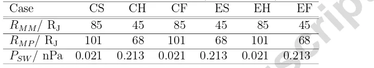
in the above studies, conductances in this region may be enhanced, above background levels, by FACs (Nichols and Cowley, 2004). Table 1 shows the three different height-integrated Pedersen conductance regions employed in our model, their corresponding ionospheric latitudes and their assigned
val-ues of ΣP. Section 6.4 discusses the limitations in using such assumptions.
3.3. Magnetosphere model
The axisymmetric Jovian magnetosphere model employed in this study is the same as that described in Yates et al. (2012). It combines a detailed model of the inner and middle magnetosphere (Nichols and Cowley, 2004) with a simplified model of the outer magnetosphere and region of open field lines (Cowley et al., 2005). The ability to reconfigure the magnetosphere depending on its size is also included by assuming that magnetic flux is con-served (Cowley et al., 2007). Surfaces of constant flux function define shells
of magnetic field lines with common equatorial radii ρe and ionospheric
co-latitude θi. These surfaces also allow for the magnetic mapping from the
equatorial plane of the magnetodisc (middle magnetosphere) to the
iono-sphere. This mapping requires an ionospheric flux function Fi(θi), a
mag-netospheric counterpart Fe(ρe) (representing the magnetic flux integrated
between a given equatorial radial distance ρe and infinity) and the equality
Fi(θi)=Fe(ρe), which represents the mapping betweenθi andρe to which the
corresponding magnetic field line extends (Nichols and Cowley, 2004). The ionospheric flux function is given by:
Fi =BJρ2i =BJRi2sin2θi, (2)
where BJ is the equatorial magnetic field strength at the planet’s surface
and ρi is the perpendicular distance to the planet’s magnetic/rotation axis
(ρi=Risinθi, where Ri is the ionospheric radius. We adopt BJ=426400 nT
(Connerney et al., 1998), and Ri=67350 km (Cowley et al., 2007). Note
Ri<RJ due to polar flattening at Jupiter. For further details on the
3.4. Obtaining the transient plasma angular velocity
In steady state, plasma angular velocity profiles are obtained in a simi-lar manner to that discussed in Smith and Aylward (2009) and Yates et al. (2012); by solving the Hill-Pontius equation in the inner and middle magne-tosphere, but assuming a constant Pedersen conductance.
We now discuss the calculation of plasma angular velocity once the model has entered the transient regime i.e. once our initial, steady-state system be-gins to undergo a transient compression/expansion of the magnetosphere. Our method of calculating transient plasma angular velocities follows that of Cowley et al. (2007). Prior to the rapid compression or expansion, the
system exists in a steady state, with plasma angular velocity ΩM(θi, t=0)
as a function of co-latitude θi and time t. Using the magnetic mapping
method discussed in section 3.3, the equatorial radial distance ρe(θi, t=0)
of the local field line can be found. The arrival of the solar wind pulse or rarefaction causes the magnetosphere to compress or expand by several tens
of RJ (typical choice for the simulations) and the model enters the transient
(time-dependent) regime. Thus, a given co-latitudeθi now maps to a new
ra-dial distanceρe(θi, t). If, as discussed in section 2, the solar wind pulse causes
perturbations that occur on sufficiently small time scales (∼2−3 hours), we
can assume that plasma angular momentum is approximately conserved. The plasma angular velocity profile throughout the ‘pulse’ in solar wind pressure is then given by:
ΩM(θi, t) =ΩM(θi, t=0)
ρe(θi, t=0) ρe(θi, t)
2
, (3)
where the notation t=0 andt denote the initial (steady-state) and transient
state (at each time-step throughout the event) respectively.
For this study, the time evolution of solar wind dynamic pressure, and
thus magnetodisc size, is represented by a Gaussian function. RMM(t)
rep-resents the magnetodisc radius as a function of time and is given by
RMM(t) =Ae−
(t−to)2
whereA=RMM(to)−RMMOand is the amplitude of the corresponding curve,
RMMO is the initial magnetodisc radius, RMM(to) is the maximum or
min-imum radius, to is the time at which RMM(t)=RMM(to) (90 minutes after
pulse start time ts), and Δt controls the width of the ‘bell’ (obtained
us-ing (2/3)(to−ts) = 2√2 ln 2 Δt ). After achieving steady-state, we run the
model for a single Jovian day, transient mode is then initialised 3 hours prior
to the end of the Jovian day (and model runtime). Profiles of RMM(t) for
compressions and expansions are shown in Fig. 1.
As indicated in Fig. 1, the simulated pulse lasts for a total of three hours, after which the magnetodisc returns to its initial size. This is represented by the red (compression) and green (expansion) lines. The black dashed line
indicates the point of maximum compression/expansion (at t=to) where we
take a ‘snapshot’ of model outputs in order to investigate the thermospheric response midway through the transient pulse (henceforth, this phase of the event is referred to as ‘half-pulse’).
As in Yates et al. (2012), we divided the magnetosphere into four regions: region I, representing open field lines of the polar cap; region II containing the closed field lines of the outer magnetosphere; region III (shaded in figures) is the middle magnetosphere (magnetodisc) where we assume the Hill-Pontius equation is valid for steady-state conditions. Region IV is the inner magne-tosphere (which is assumed to be fully corotating in steady state). Region III is our main region of interest throughout this study since it plays a central role in determining the morphology of auroral currents.
and deep planet creates a reversal of currents and angular momentum trans-fer between the ionosphere and magnetosphere (Cowley et al., 2007). Thus angular momentum is transported from the magnetosphere to the thermo-sphere, where rotation rate increases from its initial state. We see an average
of ∼3 % increase in peak ΩT in response to the transient compression event.
This is small compared to the factor of two increase in peak ΩM (for case
CH). The significant difference in response between the thermosphere and magnetosphere is due to the larger mass of the neutral thermosphere and thus, its greater resistance to change (inertia). After the subsidence of the
pulse, the magnetosphere returns to its initial size and, thus, the ΩM profile
for case CF is equal to that of CS at all latitudes. The same cannot be said for the thermospheric angular velocities; the CF thermosphere rotates
slightly faster (∼2 % at maximum ΩT) for parts of regions III and I and all
of region II. This comparison highlights the difference in response between the thermosphere and magnetosphere to the prescribed changes in solar wind pressure.
Fig. 2b shows angular velocity profiles corresponding to the transient expansion scenario. Like the compression scenario, we have cases ES
(pre-Expansion Steady-state (initial value ofRMM=45RJ)), EH (Expansion
Half-pulseRMM=85RJ) and EF (Expansion Full-pulse) indicated by blue, red and
green lines respectively. The behaviour is very different from the compression: midway through the event (case EH), the magnetodisc plasma sub-corotates to an even greater degree in regions IV and III compared to the initial steady-state case, ES. The thermosphere also sub-corotates to a greater degree, but maintains a higher angular velocity than the disc plasma, meaning that cur-rent reversal does not occur. Thermospheric angular velocities for cases ES and EF differ slightly, as in the compression scenario i.e due to the greater lag in the thermospheric response time.
Fig. 2 theoretically demonstrates the effect that transient shocks and rarefactions in the solar wind have on both plasma and thermospheric angular
velocities. Sections 4 and 5 will discuss the effects on the M-I coupling
4. Magnetospheric Compressions
In this section we present findings for our transient magnetospheric com-pression scenario which lasts for a total of three hours.
4.1. Auroral currents
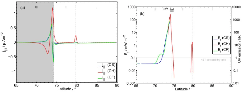
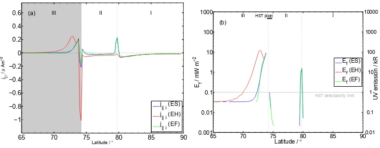
Fig. 3a shows FAC density as a function of latitude (computed from
the horizontal divergence of IP (ionospheric Pedersen current density); see
Eq. (A.3)) for cases CS, CH and CF. The blue line represents case CS, whilst the red and green lines respectively show cases CH and CF. Both cases CS and CF possess upward (positive) FAC density (indicating downward
mov-ing electrons) peakmov-ing at ∼74◦, corresponding to the ‘main auroral oval’.
Strong downward (negative) FAC densities are located at the region III/II boundary, indicating that electrons in this region are moving upwards along the magnetic field lines. In regions II and I, FAC density profiles remain slightly negative. Peaks in upward FAC arise from strong spatial gradients
in ΩM (ΩM decreases by∼78 % across∼2◦caused by the breakdown in
coro-tation of magnetodisc plasma), and consequently, flow shears located at or near magnetospheric region boundaries. Downward FACs at the region III
boundary are also caused by large spatial gradients in ΩM and to a lesser
extent the change in ΣP encountered as we traverse this boundary (Yates
et al., 2012). The minor differences between these two cases are attributed to the response of the thermosphere to the transient pulse. At full-pulse,
ΩM(CF)=ΩM(CS) but ΩT(CF)=ΩT(CS) as the thermosphere has not had
sufficient time to settle back to a steady-state (due to its large inertia, as dis-cussed in section 3.4). Although this is a subtle example of the atmospheric modulation of auroral currents, future simulations will aim at further explor-ing how this effect changes within the parameter space of the pulse duration and its change in solar wind pressure.
Case CH shows the largest deviation from steady state. Its FAC density
profile is directed downwards at latitudes up to ∼73◦. This current reversal
(compared to case CS) is due to a negative flow shear (ΩT −ΩM) caused by
i)the ’main auroral oval’: where a peak upward FAC density of∼1.2μA m−2 (a factor-of-two increase compared to case CS) is due to magnetodisc plasma transitioning from a super-corotational state to a significantly sub-corotational state.
ii)the region II/I (open-closed field line) boundary: with an upward FAC
density peak of∼0.2μA m−2caused by the differing ΩM in these two regions.
In region II ΩM is fixed at a value depending on magnetodisc size (Cowley
et al., 2005). In region I, we set ΩM = 0.10 ΩJ, for all cases, in accordance
with the formula of Isbell et al. (1984).
We briefly compare FAC densities from case CH with transient results
from Cowley et al. (2007) (compression from 85−45 RJ). Despite a
resem-blance in FAC profiles, upward FACs in the magnetodisc (region III) are
∼2.5 times larger in case CH than the equivalent case (with a responsive
thermosphere) in Cowley et al. (2007). FACs in case CH are actually closer to those in Cowley et al. (2007)’s non-responsive thermosphere compression case. This suggests that, the thermosphere (represented by a GCM) in our study lies somewhere in between a responsive and non-responsive thermo-sphere (although closer to the latter, for the pulse parameters assumed).
Corresponding precipitating electron energy fluxes are shown in Fig. 3b. These fluxes are plotted as a function of latitude and obtained using Eq. (B.1) and Table B.1, which uses only the upward (positive) FAC densities pre-sented in Fig. 3a. The line style code and labels are the same as in Fig. 3a. The latitudinal size of a Hubble Space Telescope (HST) ACS-SBC pixel
(0.03x0.03 arc sec) is represented by the dark grey rectangle (assuming that
the magnetic axis of the Jovian dipole is perpendicular to the observer’s line of sight) and the grey solid line indicates the limit of present
detectabil-ity with HST instrumentation (∼1 kR; Cowley et al. (2007)). We initially
compare electron energy fluxes for cases CS and CF. These profiles are
non-existent poleward of ∼74◦; equatorward of this location, case CF shows
little deviation from CS, except that caused by the thermospheric lag dis-cussed above. In region III, we find that the peak energy flux for case CF is
∼35 % larger than that in case CS and the location of these peaks coincide
with the location of the main auroral oval (∼74◦). The slight increase in
peak energy flux is due to a relative increase in flow shear as seen in Fig. 2a.
brighter than that of CS as indicated by the right axis in the Figure
(assum-ing that 1 mW m−2 of precipitation creates ∼10 kR of UV output (Cowley
et al., 2007)).
The Ef profile for case CH is different from those of both cases CS and
CF. There are three main changes in CH compared to CS: i) peak energy
flux in region III is ∼280 mW m−2, almost a factor of five larger,ii) location
of peak energy flux has shifted polewards by ∼0.2◦ and, iii) presence of a
second peak with an energy flux of 1.7 mW m−2 at the region II/I boundary.
The large increase in electron energy flux is caused by a substantial increase in flow shear between the thermosphere and magnetosphere, resulting from the super-corotation of the magnetodisc plasma (see Fig. 2). The presence of a second upward FAC region at the region II/I boundary is also due to flow shear increase across the boundary, as the magnetosphere in region II
corotates at a larger fraction of ΩJ compared to case CS. The result for this
higher-latitude boundary should be regarded as preliminary, since it is
sensi-tive to the values of ΩM we assume in the outer magnetospheric region and
polar cap. Flow velocities in these regions are poorly constrained, with few
observations (Stallard et al., 2003). The increase in Ef for case CH would
lead to corresponding increases in auroral emission. As such, we would
ex-pect ‘main oval’ emission for case CH to shift polewards by ∼0.2◦ and be
∼4.7×larger than emission in case CS i.e. ∼2800 kR compared to∼600 kR.
Comparing the energy flux profile of case CH with the equivalent case in Cowley et al. (2007), we see that in the closed field regions (III and II), peak energy fluxes are two orders of magnitude larger in case CH. This demonstrates the differences between using a GCM to represent the ther-mosphere and using a simple ‘slippage’ relation between thermospheric and magnetospheric angular velocities. At the open-closed field line boundary (II/I boundary) our peak flux is an order of magnitude smaller than that in Cowley et al. (2007); this difference arises from the different models used to represent the outer magnetosphere. The outer magnetosphere (region II) and open field line region (region I) in this study is modelled using plasma angular velocities from Cowley et al. (2005).
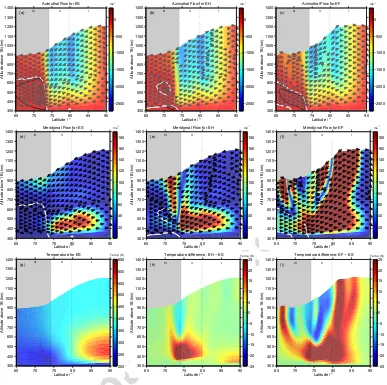
4.2. Thermospheric dynamics
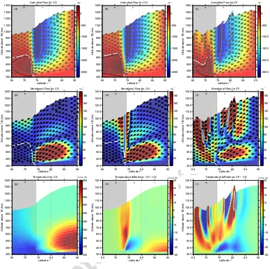
Figs. 4a-c show the variation of thermospheric azimuthal velocity (in the corotating reference frame) in the high latitude thermosphere for cases CS-CF respectively. Positive (resp. negative) values of azimuthal velocity indicate super (resp. sub)-corotating regions. The direction of meridional flow is indicated by the black arrows, the locus of rigid corotation is indicated by
the solid white line, strong super-corotation (<25 m s−1) is indicated by the
black contour, strong sub-corotation (> −2500 m s−1) is indicated by the
dashed white contour. Magnetospheric regions are labelled and separated by black dotted lines. Zonally, there are two prominent features in our transient compression cases:
i) a low altitude small super-corotating jet, centred at ∼72◦. In case
CS, this jet is created by a small excess in the zonal Coriolis and advec-tion momentum terms compared to the ion drag term. At low altitude, the Coriolis force is primarily directed eastwards and unopposed can promote super-corotation in the neutrals (Smith and Aylward, 2009; Yates et al., 2012).
ii) a large sub-corotating jet, from region III - I (blue region in Figs.
4a-c). This sub-corotational jet is caused by the drag of the sub-corotating magnetosphere on the thermosphere. Zonal flows in this region are generally sub-corotational and acceleration terms are balanced in case CS, as the ther-mosphere is in steady-state.
Figs. 4d-f shows the variation of meridional flows in the high latitude thermosphere for our transient compression cases. Magnetospheric labels, locus of corotation and arrows are the same as in Figs. 4a-c. These figures show the meridional flow patterns in the thermosphere, as well as localised accelerated regions (red/brown hues). In steady state, flow patterns are as described by Smith et al. (2007), Smith and Aylward (2009) and Yates et al. (2012) - where at:
i) Low-altitude (<600 km), ion drag acceleration becomes strong due
to the Pedersen conductivity layer (maximum value of 0.1163 mho m−1 at
∼370 km). An imbalance is created between ion drag, Coriolis and
pres-sure gradient terms; thus, giving rise to advection of momentum, which re-stores equilibrium in this low altitude region. This results in mostly sub-corotational, poleward accelerated flow as shown by the black arrows and brown hues in Fig. 4d.
Coriolis and pressure gradient accelerations are essentially balanced, whilst terms such as ion drag, advection and zonal Coriolis are small and insignif-icant. This creates a ‘jovistrophic’ condition, whereby flow is directed very slightly equatorwards and is sub-corotational (see black arrows in Fig. 4d).
The above descriptions of zonal and meridional flow patterns pertain to steady state conditions (Figs. 4a and d respectively). Zonal flows for case CH (Fig. 4b) show little change from the steady state zonal flow patterns described above. The main differences lie in the magnitude of the velocities; velocity in the super-corotational jet doubles and the magnitude of azimuthal
velocity has decreased by ∼4 % in the sub-corotational jet. Meridional flows
in Fig. 4e show two additional local acceleration regions either side of ∼73◦
latitude and from altitudes >500 km.
In addition, low altitude flow in region III is now directed purely equator-ward. This is in marked contrast to the steady state flow patterns. All the changes in flows discussed for case CH result from the super-corotation of the magnetosphere which causes a reversal in the coupling current, subsequently leading to a change in the sign of ion drag momentum terms in region III (see Fig. 9 and corresponding discussion).
Zonal and meridional flows of case CF are respectively show in Fig. 4c and f. The overall flow patterns are as described above for case CH: i) a large sub-corotational jet combined with low altitude poleward flows and high altitude equatorward flows in regions II and I, and ii) a low small low altitude super-corotational jet combined with equatorward flows in region III. However, the degree and spatial extent of super-corotation has decreased and a number of local accelerated regions exist where the direction of meridional flow changes on relatively small spatial scales. These complex flow patterns result from the highly perturbed nature of the case CF thermosphere and the imbalance between ion drag, Coriolis, pressure gradients and advection of momentum terms.
4.3. Thermospheric heating
cooling (Figs. 5d-f) terms (see plot legends for details) to interpret the tem-perature response.
In Fig. 4g we see a clear temperature difference between upper (>75◦)
and lower (<75◦) latitudes; lower latitudes are cooled whilst upper latitudes
are significantly heated (Smith et al., 2007; Smith and Aylward, 2009). We
see a ‘hotspot’ (in region I) with a peak temperature of ∼705 K. This arises
from the poleward transport of Joule heating (from regions III and II) by the accelerated meridional flows shown in Fig. 4d (Smith and Aylward, 2009; Yates et al., 2012).
Fig. 4h shows the temperature difference between cases CH and CS. There are three prominent features in Fig. 4h:
i) Temperature increase up to ∼26 K across the region III/II boundary
(z≥400 km) resulting from a large (×2 ) increase in Joule heating and the
addition of other heat sources, such as adiabatic heating (see Fig. 5b). The large increase in Joule heating is caused by the increase in the rest-frame electric field, and the corresponding Pedersen current density.
ii) Temperature decrease down to ∼−22 K, at low altitudes of region II.
Fig. 5b shows that at low altitudes (≤500 km) of region II there is, on average,
a 20 % decrease in energy dissipated by Joule heating and ion drag energy. This, coupled with the presence of energy lost by ion drag energy (Fig. 5e) in this region causes the significant decrease in temperature shown above. All the factors discussed above result from the reversal and decrease (in magnitude) of the flow shear between the magnetosphere and thermosphere in case CH.
iii)A maximum of∼17 K increase at low altitudes in region I. The
merid-ional velocity of case CH increases slightly (∼2 %) in this region and, as such,
can transport heat from Joule heating and ion drag energy polewards some-what more efficiently than in case CS.
Fig. 4i shows the temperature difference between cases CF and CS. Imme-diately, we can see that there are changes in the distribution of temperature in the upper thermosphere of case CF. There are four ‘finger-like’ regions
with local temperature increases ≥50 K (maximum of 175 K; white contour
encircles regions where temperature difference is ≥100 K) and three regions
devia-tions increase with altitude and are collocated with accelerated meridional flow regions. Considering Figs. 5c and f, we see that the heating and cooling terms are now quite complex, with advective and adiabatic terms
dominat-ing (≥10×Joule heating and ion drag energy terms). The CF thermosphere
appears to be transporting heat, both equatorward and poleward from the region III/II boundary (see Fig. 4f). Achilleos et al. (1998) also shows a sim-ilar phenomenon (see top left of Fig. 9 in Achilleos et al. (1998)), whereby perturbations of high temperature are transported away from the auroral re-gion by meridional winds. The energy deposited in the auroral rere-gions heats the local thermosphere which increases local pressure gradients. Advection then attempts to redistribute this heat which momentarily cools the local area until enough heat is deposited again and the process restarts.
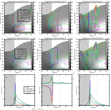
Figs. 5g-i show powers per unit area as functions of ionospheric latitude for cases CS, CH and CF, respectively (calculated using Eqs. (A.7 - A.11)). Blue lines represent total power transferred to the ionosphere from planetary rotation which is divided into the power used to accelerate the magneto-spheric plasma (magnetomagneto-spheric power; red lines) and power dissipated in the thermosphere (for atmospheric heating and changing kinetic energy; green lines). Atmospheric power is subdivided into Joule heating (black lines) and ion drag energy (cyan lines). In case CS, magnetospheric power is dominant
up to ∼73◦, where atmospheric power quickly dominates for all poleward
latitudes (see Fig. 5g). This indicates that a relatively expanded M-I sys-tem (in steady-state) generally dissipates more heat in the atmosphere than in acceleration of outward-moving plasma (Yates et al., 2012). In case CF, powers per unit area closely resemble those for case CS. There are increases
in peak magnetospheric power (∼10 %) and Joule heating (∼25 %) leading
to an overall maximum increase in available power of ∼10 %. This increase
in total power is ultimately due to the lag in response of the thermosphere. For case CH, Fig. 5h, we see the effects of plasma super-corotation in region III, where magnetospheric power reverses (now negative) and energy is now transferred from magnetosphere to thermosphere. As a consequence, heat dissipated as Joule heating doubles, positive ion drag energy decreases by
∼70 % and negative ion drag energy increases by two orders of magnitude.
5. Magnetospheric Expansions
This section presents our findings for a transient magnetospheric expan-sion event with a three hour duration.
5.1. Auroral currents
FAC densities in the high latitude region are plotted for cases ES (blue line), EH (red line) and EF (green line) in Fig. 6. Comparing cases ES with EH we see three main differences: i) EH has two upward FACs peaks in re-gion III (of similar magnitude to the peak in case ES) creating a large area of upward-directed FAC, ii) the magnitude of downward FAC near the region III boundary has increased by a factor of four (from ES to EH) and iii) FAC den-sities at the region II/I boundary are entirely downward-directed, unlike case ES. As the magnetosphere expands, its magnetic field strength and plasma
angular velocity decrease. This change in ΩM (see Fig. 2b) increases the
flow shear between the magnetosphere and thermosphere and thus increases
the FAC density in region III by ∼15 %. The strong downward FAC results
from the large gradients in ΩM through the poleward boundary of region
III, where magnetodisc plasma moves from a region with angular velocity of
0.9 ΩJ to a region moving at 0.2 ΩJ. The lack of a peak at the region II/I
boundary is due to the small change in ΩM as the model traverses these two
regions. Case EF shows only small differences with case ES due to the lag in response time of the thermosphere to transient magnetospheric changes on this time scale.
Looking now at case EH, and comparing FAC densities with the
corre-sponding result from Cowley et al. (2007) (expansion from 45−85 RJ), we
notice a few differences: i) the magnitude of peak upward FAC in case EH is
∼25 % larger than that in Cowley et al. (2007) and, ii) case EF has no upward
FAC at the region II/I boundary, contrary to results in Cowley et al. (2007). These differences emphasise the effect of using a time-dependent GCM for the thermospheric response. For example, the ‘double peak’ structure in the upward Region III FACs is due to additional modulation of current density by thermospheric flow.
the latitudinal size of a HST ACS-SBC pixel is indicated by the dark grey rectangle and the grey solid line indicates the limit of present HST
detectabil-ity (∼1 kR; Cowley et al. (2007)). We begin by comparing profiles for case ES
with EF, which are almost identical and both have maxima at∼74◦ latitude,
equivalent to the location of the ‘main auroral oval’, and at∼80◦, the
bound-ary between open (region I) and closed field lines (region II). Therefore, we
would expect a fairly bright auroral oval of ∼88 kR for case ES and∼79 kR
for case EF. The electron energy flux for case EF (∼7.85 mW m−2) is ∼10 %
smaller than case ES (∼8.8 mW m−2) due to ΩT(ES)>ΩT(EF) leading to
a smaller flow shear. Our model also predicts the possibility of observable
polar emission (region II/I boundary) of ∼15 kR for both cases ES and EF.
However, this region is strongly dependent on the plasma flow model used and poorly constrained by observations.
Energy flux Ef for case EH is non-existent, poleward of ∼74◦ latitude,
due to the downward (negative) FAC density in this region. In region III,
there are two upward FAC peaks, separated by ∼1◦. The first one, located
at ∼73◦ is ∼37 % larger than the second, at∼74◦. These peaks result from
the large degree of magnetospheric sub-corotation and the modulation of the thermospheric angular velocity in region III (evident in Fig. 2b). Comparing case EH with the equivalent expansion case in Cowley et al. (2007); case
EH, in region III, has a maximum value ofEf (∼12.6 mW m−2) that is twice
that in Cowley et al. (2007). This study represents the thermosphere with
a GCM which responds self-consistently to time-dependent changes in ΩM
profiles. Our results indicate that this response is not as strong as that in Cowley et al. (2007), who use a simple ‘slippage’ relation to model the thermospheric angular velocity. At the open-closed field line (region II/I) boundary, Cowley et al. (2007) obtain larger energy fluxes due to their large
change in ΩM across these regions; in our study, we obtain negligible changes
in Ef due to our smaller change in imposed ΩM across this boundary.
5.2. Thermospheric dynamics
For case ES, the zonal (Fig. 7a) and meridional (Fig. 7d) flows are very similar to those discussed in Yates et al. (2012) as the only difference between both steady-state compressed cases is that here we assume a constant height-integrated Pedersen conductivity whilst in Yates et al. (2012) the conductiv-ity is enhanced by FAC. Zonal flows show a low-altitude super-corotational jet in region III and two sub-corotational jets across regions II and I. The meridional flows show the previously discussed flow patterns i.e. low-altitude poleward flow and high-altitude equatorward flow.
Thermospheric flows for case EH are slightly different from those of case ES. A magnetospheric expansion decreases the degree of plasma corotation which subsequently decreases the thermospheric zonal velocities i.e. they be-come more sub-corotational (see Fig. 7b). In the meridional sense (Fig. 7e), low altitude flows remain poleward but with an increased magnitude (up to
∼30 %) and all flow in region II is now directed poleward. Extra heating
(see section 5.3) near the region III/II boundary causes the forces in the lo-cal thermosphere to become unbalanced leading to accelerated flows in the poleward and equatorward (high-altitude of region III) directions.
The thermospheric velocities at the end of the transient expansion event (case EF) are shown in the third column of Fig. 7. We see that the only change in zonal flow patterns is a slight increase in the zonal velocity (al-gebraic increase). The meridional winds show a large poleward accelerated flow originating at low altitudes in region III and reaching the high altitudes of region I. Two smaller regions of accelerated equatorward flow arise in the upper altitudes of regions III and II. As the magnetosphere returns to its initial configuration, it weakly super-corotates over most of region III; this transfers angular momentum to the sub-corotating thermosphere which acts to ‘spin up’ the thermospheric gas.
5.3. Thermospheric heating
(see plot legends for details).
Fig. 7g shows similar results to those described in section 4.3. The main difference is related to the polar ‘hotspot’ which is considerably cooler (peak
temperature of ∼590 K) than that for case CS (peak temperature ∼705 K).
As previously discussed, the ‘hotspot’ results from the meridional trans-port (via poleward accelerated flows) of Joule heating from lower latitudes
(∼73−84◦; see Figs. 7d and 8a) (Smith and Aylward, 2009; Yates et al.,
2012).
Fig. 7h exhibits the temperature difference between cases EH and ES.
The figure shows a maximum of∼50 K temperature increase at low altitudes
(<700 km) in regions III and II. Also evident are two minor temperature
variations: i) ∼10 K decrease at high altitude, centred on the region III/II
boundary and, ii) ∼10 K increase in the polar ‘hotspot’ region. Fig. 8b
shows a large (≥4×) increase in ion drag energy and Joule heating rates
which accounts for the temperature increase across regions III and II. This low-altitude increase in temperature causes a local increase in pressure gradi-ents leading to accelerated meridional flows being able to efficiently transport heat away from the region III/II boundary and towards the pole. The high altitude cool region ensues from local equatorward and poleward meridional flows combined with factor-of-three increase in adiabatic cooling (Fig. 8e).
Fig. 7i shows the temperature difference between cases EF and ES. The temperature profile has changed significantly from that in Fig. 7h. There are
two regions where temperatures increase by up to ∼50 K: i) extending from
∼73−85◦ latitude and low altitudes in regions III and II, and all altitudes
in region I (these map to the large poleward-accelerated region in Fig. 7f);
and ii) high-altitude (>600 km) region, centred at ∼66◦ latitude. These
re-gions are primarily heated by horizontal advection (high-altitude only) and adiabatic terms (all altitudes) as shown in Fig. 8c; these heating rates have increased (from case ES) by, at most, 800 % and 500 % respectively. The
final feature of note in Fig. 7i is the region cooled by up to ∼−22 K,
ly-ing between the two heated regions at altitudes >550 km. This cooling is
Figs. 8g-i show powers per unit area as functions of ionospheric latitude for cases ES-EF respectively. Colour codes and labels are as in Figs. 5g-i. Fig. 8g shows the energy balance in the thermosphere for case ES. As dis-cussed in Yates et al. (2012), most of the energy in region III is expended in accelerating magnetospheric plasma; in region II we have a situation where magnetospheric power and atmospheric power (the sum of Joule heating and
ion drag energy) are equal, due to ΩM=0.5 ΩJ. Atmospheric power is
domi-nant in region I. For case EH (Fig. 8h), the magnetodisc plasma sub-corotates to a large degree which causes the majority of available power to be used in
accelerating the sub-corotaing plasma. Poleward of∼73◦ latitude, the large
flow shear (ΩT −ΩM) leads to an increase in energy dissipated within the
thermosphere, primarily through Joule heating. The magnetosphere of case
EF super-corotates, compared to the thermosphere, at latitudes ≤73◦. This
causes a reversal in energy transfer, which now flows from magnetosphere to atmosphere and acts to spin up the sub-corotaing neutral thermosphere (see
Fig. 8i). Polewards of 73◦, the energy balance is similar to that of case ES.
6. Discussion
6.1. Effect of a non-responsive thermosphere on M-I coupling currents
Our work makes no a priori assumptions regarding the response of the thermosphere to magnetospheric forcing. The GCM responds self-consistently by solving the Navier-Stokes equations for momentum, energy and continu-ity. For completeness, we calculated M-I coupling currents for the case of a non-responsive thermosphere (Gong, 2005). To do this, we assume that
ΩT=ΩT(CS) throughout the entire transient event. In this non-responsive
thermosphere scenario, there is an average increase in M-I currents of∼20 %
midway through the pulse compared to case CH (obtained using GCM). At full-pulse, however, the non-responsive case has M-I currents that are on
average ∼12 % smaller than currents in case CF. These differences between
a non-responsive thermosphere and a responsive one (GCM), are related to the flow shear between thermosphere and magnetosphere; which, is maximal (resp. minimal) at half-pulse (resp. full-pulse) when using a non-responsive thermosphere. A similar analysis for the expansion scenario results in an
average of ∼20 % increase in the maximum magnitude of M-I currents in a
non-responsive thermosphere, compared to the GCM thermosphere. Here,
flow shear in the non-responsive scenario will always be greater than the flow shear obtained with the GCM thermosphere.
6.2. The auroral response: predictions and comparisons with observations
Figs. 3b and 6b respectively show the change in precipitating electron en-ergy flux in response to transient magnetospheric compression and expansion events. We also indicate (on the right axis of these Figures) the corresponding
UV emission associated with such energy fluxes (assuming that 1 mW m−2
of precipitation creates ∼10 kR of UV output). Considering the compression
scenario, our results suggest that the arrival of a solar wind shock would
in-crease the UV emission of the main oval from ∼600 kR to ∼2800 kR (factor
of 4.7 ) and constrict the width of the oval by ∼0.2◦. The HST
detectabil-ity limit and the size of an HST pixel (dark grey box in Fig. 3b) suggest that such an increase in auroral emission would be detectable but the con-striction of the main oval may be too small to be observed. Clarke et al. (2009) and Nichols et al. (2009) observed that the brightness of UV auro-ral emission increased by a factor of two, in response to transient (almost
instantaneous) increases in solar wind dynamic pressure (∼0.01−0.3 nPa or
equivalently ∼109−72 RJ). The increase in UV emission was also found to
persist for a few days following the solar wind shock. Nichols et al. (2009) also observed poleward shifts (constrictions) in main oval emission on the
order of ∼1◦ corresponding to the arrival of solar wind shocks.
Total emitted UV power may also be used to describe auroral activity,
assuming that this quantity is ∼10 % of the integrated electron energy flux
per hemisphere (Cowley et al., 2007). Case CH has a total UV power of
∼1.58 TW (compared to ∼420 GW for case CS), which is a factor of two to
three times larger than UV powers observed by both Clarke et al. (2009) and Nichols et al. (2009). The profile of case CH also indicates the possibility of observable polar emission at region II/I (open-closed) boundary. This con-clusion is, however, sensitive to our model assumptions (see section 6.4).
Our model results predict very different behaviour for the expansion sce-nario (Fig. 6b). At maximum expansion we would expect a small increase
(∼40 kR) in peak main oval brightness along with a ∼1◦ equatorward shift
∼73◦ and ∼74◦ latitude. The main oval would, either way, appear
consider-ably broader (∼2−3◦) as a result of the large increase in the spatial region of
magnetospheric sub-corotation. Clarke et al. (2009) observed little change in auroral brightness near the arrival of a solar wind rarefaction region, however Nichols et al. (2009) have seen changes in main oval location. The total UV
power in case EH is∼270 GW (compared to∼78 GW in case ES). While this
power is considerably smaller than that in case CH, it is comparable to UV powers calculated in Clarke et al. (2009) and Nichols et al. (2009), following
solar wind rarefactions (∼200−400 GW).
6.3. Global thermospheric response
The arrival of solar wind shocks or rarefactions has, for the most part, a similar effect on thermospheric flows. Our modelling shows a general increase (resp. decrease) in the degree of corotation with solar wind dynamic pressure increases (resp. decreases). Zonal flow patterns remain essentially unchanged with a large sub-corotational jet and a small super-corotational jet. Merid-ional flow cells however, respond to transient magnetospheric reconfigurations somewhat chaotically, with numerous poleward and equatorward accelerated
flow regions developing (at altitudes > 600 km) with time throughout the
event. The overall low-altitude poleward flow remains fixed with solar wind rarefactions but reverses in response to a solar wind shock (see cases CH and CF in Figs. 4e and f). This flow becomes equatorward due to a reversal in the direction of ion drag acceleration in the region III, as shown in Fig. 9. This reversal, in turn, arises from the super-corotation of magnetospheric plasma.
magnetosphere. This implies that its dynamics and energy input are gener-ally smaller than the transient compression scenario, which leads to a less ‘drastic’ response.
The magnetospheric reconfigurations discussed above have been shown to have a significant impact on the dynamics and energy balance of the ther-mosphere. We now attempt to globally quantify such changes in energy by calculating the integrated power per hemisphere obtained from the power densities in Figs. 5g-i and 8g-i. These integrated powers are presented in Figs. 10a and b for the compression and expansion scenarios respectively. Blue bars represent the kinetic energy dissipated by ion drag, green bars in-dicate Joule heating, red bars represent the power used to accelerate magne-tospheric plasma and orange bars simply represent the sum of all the above terms. Positive powers indicate energy dissipated in/by the thermosphere whilst negative powers indicate energy deposited into the thermosphere.
Midway through the compression event (case CH), magnetospheric plasma super-corotates compared to the thermosphere and deep atmosphere. This reverses the direction of momentum and energy transfer so that energy is now being transferred from the magnetosphere to the thermosphere. Our results
indicate that ∼2000 TW of total power (magnetospheric, Joule heating and
ion drag energy) is gained by the coupled system as a result of plasma
super-corotation. Note that this is considerably larger than the ∼325 TW (closed
and open field regions) calculated in Cowley et al. (2007) for a responsive thermosphere scenario. This energy transfer from the magnetosphere would act to, essentially ‘spin up’ the planet (Cowley et al., 2007) and increase the thermospheric temperature. In case CF, plasma is not super-corotating; thus the picture is fairly similar to case CS. The main difference is that there is
a ∼20 % increase in total power dissipated in the atmosphere and in
accel-eration of the magnetosphere. This arises from increases in flow shear due to the ‘lagging’ thermosphere (see Fig. 2) and inevitably leads to the local temperature increases seen in Fig. 4i and discussed above. The finite time required for thermospheric response results in the described ‘residual’ per-turbations to the initial system (CS) even after the pulse has subsided (CF).
A transient magnetospheric expansion event creates a significant increase
in both power dissipated in the atmosphere due to Joule heating (∼6× that
to accelerate the magnetosphere towards corotation is ∼7× that of ES, and is shown in Fig. 10b. These increases lead to a total power per hemisphere
of ∼2600 TW which is three times larger than the responsive thermosphere
case in Cowley et al. (2007). These changes in heating and cooling create the local temperature increases discussed above. For case EF, where we now have the magnetosphere rotating faster than the thermosphere, there is a
∼75 % decrease in the magnitude of ‘magnetospheric’ power. The
magne-tosphere is thus transferring power to the thermosphere in this case, albeit a relatively small amount. This effectively ‘pulls’ the thermosphere along, increasing its angular velocity in order to return to the steady-state
situa-tion where ΩT>ΩM. We note that energy dissipated via Joule heating also
decreases slightly due to the small decrease in flow shear. Overall, then, the total power per hemisphere in case EF is only 30 % that of case ES.
Results for cases CH and EH show large (approximately three orders of magnitude larger than solar heating) increases in energy either being de-posited or dissipated in the thermosphere. Observations by Stallard et al. (2001, 2002) of an auroral heating event at Jupiter were ananlysed by Melin et al. (2006). These authors found that during this auroral heating event, which they attribute to being caused by a decrease in solar wind dynamic pressure, the combined ion drag energy and Joule heating rates increase from
67 mW m−2 to 277 mW m−2 over three days. They proposed that this extra
heat must then be transported equatorward from the auroral regions by an increase in equatorward meridional winds (Waite et al., 1983). If we assume
that their auroral region ranges from 65◦ to 85◦ latitude and that these
heating rates are constant across such a region, the total energy dissipated
by Joule heating and ion drag energy increases from∼193 TW to ∼800 TW.
This increase is comparable to the increase of Joule heating and ion drag
energy in our expansion scenario, going from case ES (∼201 TW) to EH
(∼942 TW). Increase in Joule heating and ion drag energy from case CS to
CH is more modest (∼499 TW to ∼555 TW) due to the reversal of kinetic
6.4. Model limitations
The main limitation to our transient model is the use of a fixed model for relative changes in conductivity with altitude, and a uniform Pedersen
conductance ΣP for the ionosphere (see section 3.2). Whilst not ideal, we feel
it is a suitable first step to developing a fully self-consistent, time-dependent model of the Jovian magnetosphere-ionosphere-thermosphere system. Use of an enhanced conductivity model would concentrate all but background levels of conductance just equatorward of the main auroral oval location
(∼74◦) (Yates et al., 2012); effectively increasing the coupling between the
atmosphere and magnetosphere in this region. We would thus expect the magnitude of current densities to increase in the region near the main oval (region III/II boundary in our model), along with an increase in the Joule heating rate.
The high conductivity at latitudes between 60◦ and 70◦ in the present
model, combined with the super-corotation of the thermosphere, allows for the plasma magnetically mapped to these ionospheric latitudes to super-corotate slightly in steady state. With an enhanced conductivity model, this region would have a super-corotating thermosphere but low, background-level conductances (e.g. Smith and Aylward (2009); Yates et al. (2012)). There-fore, even though the super-corotating thermosphere acts to accelerate the magnetodisc plasma, the low conductances inhibit how efficiently the plasma is accelerated. It is worth noting that despite the fact that, in this study, both the neutral thermosphere and magnetodisc plasma super-corotate compared to the deep atmosphere, as long as the plasma sub-corotates compared to the thermosphere, angular momentum and energy will be transferred from the upper atmosphere to the magnetosphere as is expected in steady state. We plan to incorporate enhancements in Pedersen conductance due to auroral precipitation of electrons in a future study.
Other limitations to this model include:
i) Assumption of axial symmetry: Discussions in Smith and Aylward (2009) conclude that the assumption of axial symmetry with respect to the planet’s rotation axis does not significantly alter the thermospheric outputs of our model. They find that axial symmetry leads to modelling errors on the