BIROn - Birkbeck Institutional Research Online
Kim, Y. and Kumbhat, M. and Nagy, Z.L. and Patkos, B. and Pokrovskiy,
Alexey and Vizer, M. (2015) Identifying codes and searching with balls in
graphs. Discrete Applied Mathematics 193 , pp. 39-47. ISSN 0166-218X.
Downloaded from:
Usage Guidelines:
Please refer to usage guidelines at or alternatively
Identifying codes and searching with balls in graphs
Younjin Kim
∗Mohit Kumbhat
†Zolt´
an L´
or´
ant Nagy
‡Bal´
azs Patk´
os
§Alexey Pokrovskiy
¶M´
at´
e Vizer
kSeptember 28, 2018
Abstract
Given a graph G and a positive integerR we address the following combinatorial search theoretic problem: What is the minimum number of queries of the form “does an unknown vertexv∈V(G) belong to the ball of radiusraroundu?” withu∈V(G) and
r≤Rthat is needed to determinev. We consider both the adaptive case when thejth query might depend on the answers to the previous queries and the non-adaptive case when all queries must be made at once. We obtain bounds on the minimum number of queries for hypercubes, the Erd˝os-R´enyi random graphs and graphs of bounded maximum degree .
Keywords: identifying codes, combinatorial search, hypercube, Erd˝os-R´enyi random graph, bounded degree graphs
1
Introduction
Combinatorial search theory is concerned with problems of the following type “given a finite set S and an unknown element x∈ S, find x as quickly as possible”. In order to find x, we are allowed to ask questions of the type “is x contained in a subset B ⊆ S?” for various
∗Department of Mathematical Sciences, KAIST, 291 Daehak-ro Yuseong-gu Daejeon, 305-701 South
Ko-rea. Email: [email protected]. The author is supported by Basic Science Research Program through the National Research Foundation of Korea(NRF) funded by the Ministry of Science, ICT & Future Planning (2011-0011653)
†Sungkyunkwan Unversity, Suwon, S.Korea 440-746. Email:[email protected]
‡Alfr´ed R´enyi Institute of Mathematics, P.O.B. 127, Budapest H-1364, Hungary and E¨otv¨os Lor´and
University, Department of Computer Science, H-1117 Budapest P´azm´any P´eter s´et´any 1/C. Email: [email protected]. The author was supported by the Hungarian National Foundation for Scientific Research (OTKA), Grant no. K 81310.
§MTA–ELTE Geometric and Algebraic Combinatorics Research Group, H–1117 Budapest, P´azm´any P.
s´et´any 1/C, Hungary. Email: [email protected]. Research is supported by and the J´anos Bolyai Research Scholarship of the Hungarian Academy of Sciences.
¶Methods for Discrete Structures, Berlin. Email: [email protected]
kAlfr´ed R´enyi Institute of Mathematics, P.O.B. 127, Budapest H-1364, Hungary. Email:
[email protected] Research supported by Hungarian National Scientific Fund, grant number: 83726.
B ⊆ S. There are many real-world search problems which are of this type. For example given a set of blood samples, we might want to identify one which is infected. Or given a building, we might want to determine which room a person is hiding in.
Notice that to guarantee finding the unknown element xin a setS we always need to ask at least log2|S|questions. Indeed, to be able to distinguish between two elements x, x0 ∈S, we must at some point query a set B ⊆ S such that x ∈B and x0 6∈B. However if we ask less than log2|S| questions, then by the Pigeonhole Principle, there would be two elements
x and x0 ∈S which receive the same sequence of yes/no answers.
The lower bound log2|S| on the number of questions can be tight. In fact it is always possible to find x using dlog2|S|e questions. Indeed first we divide S is half and ask which half xis in. Then we divide the half containing x in half again, and find out which onex is in. Proceeding this way, we reduce the subset of S which x may be in by half at every step, and hence we find x after at most dlog2|S|e queries. This is the so called halving search.
Notice that in the above search the set we query at each step depends on the answers we got in the previous steps. We say that a search isadaptive if a question is allowed to depend on answers to previous questions. In practice we often would like to make all our queries at the same time (for example if each individual query takes a long time, it would save time to make queries simultaneously). We say that a search is non-adaptive if the queries do not depend on answers obtained from previous ones. Just like in the adaptive case, there exist non-adaptive searches using the optimal log2|S| number of queries. For example if S is the set of 0−1 sequences of length n, then we can find x = (x1, . . . , xn) using the n = log2|S| queries “is xi equal to zero or one?”
Note that the answers to a setQof query sets surely determine the unknown elementxif and only if for any pair of elementss1, s2 ∈Sthere exists a queryB ∈Qwith|B∩{s1, s2}|= 1. In this case we say thatB separates s1 and s2, andQis said to be a separating system or said to possess the separating property.
In this paper we study a search problem when the set S is a metric space, and we are only allowed to query setsB which are balls in the metric space. We call this theball search. There are natural search problems of this type. For example if we want to track someone moving through a building, we might set up sensors at various points in the building which tell us if the person is within a certain range. This problem is inherently non-adaptive since the person is moving (and it would usually be inpractical to change the location of the sensors as the person moves). Another example of a ball search is to locate some object in the night sky using a telescope. This problem is inherently adaptive since once we capture the object with the telescope, we would want to zoom in in order to get a better idea of its location.
Ball searches have been studied before, under the name of identifying codes on graphs. A ball Br(v) of radius r at vertex v in a graphG is the set of vertices in Gthat have distance at mostr fromv. An (r,≤l)-identifying code of the graph Gis a setC of vertices such that for every pair of distinct subsets X, Y ⊂ V(G) with |X|,|Y| ≤ l the sets Br(X)∩C and
An adaptive version of identifying codes was introduced by Moncel in his doctoral thesis [20] and in [2]. The minimum number of queries needed in the adaptive case is denoted by
a(rl)(G).
We will study a slight variant of identifying codes in which the restriction that the balls in the search must cover all the vertices of G is omitted. The reason we study this variant is that it seems to have links to a natural combinatorial object (namely the Fano Plane. See Section 2 for details). We denote by M(G, r) the minimum number of queries needed to nonadaptively find an unknown vertexv ∈Gusing balls of radius r. Similarly we denote by
A(G, r) the minimum number of queries needed to adaptively find an unknown vertexv ∈G
using balls of radius r. Notice that we always have i(1)r (G) ≤ M(G, r) ≤ i(1)r (G) + 1 and
a(1)r (G)≤A(G, r)≤a(1)r (G) + 1. Therefore, since we will mostly be interested in asymptotic estimates, it usually won’t matter whether we study the quantity M(G, r) or i(1)r (G).
Notice that in the above ball searches we specified that we could only query balls of radius exactly r. With this restriction it is not always possible to find an unknown vertex
v—for example if r is bigger than the diameter of G (the maximum distance between two vertices in G), then querying balls of radius r gives no information about the location of
v. At the 5th Eml´ekt´abla Workshop, Gyula Katona asked what happens [16] if balls of radius at most r should be allowed as queries. We’ll denote by M(G,≤ r) and A(G,≤ r) the minimum number of queries to find an unknown vertex v ∈G using balls of radius r in the nonadaptive and adaptive searches respectively. We’ll denote by M(G) and A(G) the minimum number of queries to find an unknown vertex v ∈ G using balls (of any radius) in the nonadaptive and adaptive searches respectively. Notice that since balls of radius zero are just single vertices in G, we always have M(G,≤ r), A(G,≤ r) ≤ |G|. Also, we trivially have M(G,≤ r) ≤ M(G, r) and A(G,≤ r) ≤ A(G, r). The quantities M(G,≤ r) and A(G,≤ r) are monotonic in the sense that M(G) ≤ M(G,≤ r+ 1) ≤ M(G,≤ r) and
A(G)≤A(G,≤r+ 1)≤A(G,≤r) hold for all r.
The first metric spaces in which we will study the ball search are hypercubes. Let Qn be the n dimensional hypercube—the set of all 0−1 vectors of length n. We define a graph on
Qnby placing an edge between two vectors whenever they differ in exactly one entry. In this graph the distance d(u, v) between two vertices is exactly the Hamming distance between
u and v i.e. the number of entries on which u and v differ. If c is an element of Qn and
r is a non-negative integer, then B(c, r) denotes the ball of center c and radius r, that is,
B(c, r) := {v : v ∈ Qn, d(c, v) ≤ r}. The most recent upper and lower bounds on i (l) r (Qn) were proved in [4, 8, 6, 7, 12]. Adaptive identification inQn was studied by Junnila [13] who obtained lower and upper bounds on a(1)1 (Qn). To be able to state our results let K(n, r) denote the minimum number of balls of radius r that cover all vertices of Qn. The centers of such balls are said to form covering codes in Qn [5].
Theorem 1.1. The functionsA(Qn), A(Qn,≤r)andA(Qn, r)satisfy the following
inequal-ities:
(i) n≤A(Qn)≤n−1 +dlog(n+ 1)e.
(ii) K(n, r)−1≤A(Qn,≤r)≤K(n, r) +n−1 +dlog(r+ 1)e. There is a constant C such
(iii) K(n, r)−1 ≤ A(Qn, r) ≤ K(n, r) + Pr
i=0 n r
. There is a constant C0 such that if
r≤C0n, then A(Qn, r) = (1 +o(1))K(n, r).
In Section 2, we will also study M(Qn) for small values of n.
Then we turn our attention to the Erd˝os-R´enyi random graph modelG(n, p). The asymp-totics of i(1)1 (G(n, p)) was determined by Frieze, Martin, Moncel, Ruszink´o, and Smyth [10] provided p,1−p≥4 log logn/logn holds. Using results of Bollob´as [3] and Katona [15] we obtain upper and lower bounds on M(G(n, p), r) that differ by an O(lnn)-factor for any r
that is smaller than the diameter of G(n, p) whenever p= Ω(n−1+ε). As the formulation of our theorem is somewhat technical, we defer its statement until Section 3.
Finally, we consider graphs of bounded maximum degree. Results concerning the param-eter i(1)1 (G) for such graphs, for random d-regular graphs and for some other graph classes defined by their degree sequences were obtained by Foucaud and Perarnau [9]. Let us denote byG∆,n the set of finite graphs on n vertices with maximum degree at most ∆.
Theorem 1.2. For all connected graphs G∈ G∆,n we have A(G) = Θ∆(logn).
Notice that the connectivity assumption cannot be ommited in the above theorem. In-deed, otherwiseGcould be a union of disjoint cliques on ∆+1 vertices. A search in this graph must ask at least one query in each component, and hence use at least|G|/(∆+1) =ODelta(n) queries. Similarly, the bound on the maximal degree of G cannot be removed since an op-timal search on a star with n vertices needs n−1 queries. Finally, note that Theorem 1.2 cannot be strengthened to give a logarithmic bound on the length of a non-adaptive search on bounded degree graphs. Indeed it is easy to show that M(Pn) = dn−21e, and so even for graphs with ∆ = 2 , the nonadaptive search may need linearly many queries.
Let us observe the connection of non-adaptive ball search to another well studied pa-rameter of graphs. A set D of vertices of Gis called a resolving set of Gif for any vertices
x, y ∈V(G) there existsz ∈D such thatd(x, z)6=d(y, z). The minimum size of a resolving set is called the metric dimension of G (introduced in [11, 21]) and is denoted by β(G). Clearly, if a set of ball queries finds an unknown vertex v, then the centers of the balls form a resolving set inG and thus we haveβ(G)≤M(G). Also, ifDis a resolving set in G, then the query set {BG(d, i) : d ∈ D,1 ≤ i ≤ diam(G)} finds the unknown vertex of G, where
diam(G) denotes the diameter of G. Consequently, we have M(G)≤diam(G)β(G).
Throughout the paper “log” stands for the logarithm of base 2, and “ln” denotes the natural logarithm.
2
The hypercube
In this section we consider the adaptive search on Qn. We find bounds on A(Qn) and
A(Qn,≤r). We also find a code in Q7 of balls of radius 3 that is in some sense better than the best previously known one. We start by proving Theorem 1.1.
Throughout this section we will denote the number of vertices in a ball of radius r in
Qn byV(n, r) = Pr
i=0 n r
Proof of Theorem 1.1: (i) For the lower bound notice that the sequence of answers must be different for each vertex. Therefore there must be at least log(|Qn|) = n questions. For the upper bound, let u∗ be the unknown element of Qn. We give an adaptive algorithm that finds u∗ and uses at most n−1 +dlog(n+ 1)e queries.
The first part of our algorithm uses dlog(n+ 1)e queries to determine the distance
d(0, u∗). Notice that asking a ball B(0, r) is equivalent to asking whether we have
d(0, u∗) ≤ r or d(0, u∗) > r. Note that d(0, u∗) > r can be anything in the set
{0,1, . . . n}. In the first query we ask the ball B(0,bn/2c). Depending on whether we get a “yes” or “no” answer, we obtain that d(0, u∗) is either in{0, . . .bn/2c} or in
{bn/2c+ 1, . . . , n}. Continuing in this fashion, always asking B(0, r) where r is the median of the possible (not already excluded) distance values, we see that dlog(n+ 1)e
determine d(0, u∗). Let us denote this distance by d.
To finish the algorithm we show that for every 1≤i≤none further query is enough to determine the value of u∗’sith coordinate. Indeed,u∗ ∈B(ei, d−1) holds if and only if the ith coordinate of u∗ is 1. We ask the ballsB(ei, d−1) for i= 1, . . . , n−1 in order to determine u∗1, . . . , u∗n−1. Sinceu∗n =d−Pn−1
i=1 u ∗
i, this is enough to determine u∗. (ii) For the lower bound, observe that if after asking balls B1, B2, . . . , Bt we are able to
determine the unknown vertex, then at most one vertex is not covered by the union of the balls.
For the upper bound, consider the following algorithm. First, let us ask a set of balls
B of radius r that cover all vertices and with|B| =K(n, r). After finding a ball B ∈ B
containing the marked vertex, we repeat the algorithm of part(i)with the modification that we know that the marked vertex is of Hamming distance at most rfrom the center of B. Therefore, to determine this distance exactly, we only needdlog(r+ 1)e queries. We now show that there is a constant C such that if r ≤ n/2 − C√nlogn, then
A(Qn,≤r) = (1 +o(1))K(n, r). The exact value of K(n, r) is known only for a short range of n and r and even determining the asymptotics of K(n, r) is one of the major open problems of coding theory. For an introduction to covering codes, see the book [5]. Clearly K(n, r) ≥ 2n/V(n, r) holds. It is known that for any fixed r, we have
K(n, r) = Θ(2n/V(n, r)) (the best known constant is due to Krivelevich, Sudakov and Vu [18]) and that for any function r=r(n) we have K(n, r) = O(n2n/V(n, r)).
By the above reasoning we obtained that to prove A(Qn,≤r) = (1 +o(1))K(n, r), it is sufficient to show that n=o(2n/V(n, r)) holds. This holds since we have 2n/V(n, r)≥ exp((n−2r)/√n) andr ≤n/2−C√nlogn.
(iii) The lower bound follows from part (ii). For the upper bound, proceed as we did in part (ii) to use K(n, r) queries to find one ball of radius r containing the marked vertex. After that we can eliminate one possible vertex by each further query thus finding u∗
with K(n, r) +V(n, r) queries.
We finish this section with considering the special case n = 7. There are many results on i(1)r (Qn) for small values ofr and n. In [4], Charon, Cohen, Hudry, and Lobstein proved that i(1)3 (Q7) = 8. This is true, but the lower bound is due to the fact that the definition of identifying code includes the condition that balls around the codewords should cover all vertices of the graph. On the other hand, no 7 of their 8 codewords possess the separation property. This can be checked easily as if they did, then for any two of them B(c1,3)∩
B(c2,3), B(c1,3)\B(c2,3), B(c2,3)\B(c1,3), V(Q7)\(B(c1,3)∪B(c2,3)) should have size 32 and consequently those 7 codewords should have pairwise Hamming distance 4. In the remainder of this section we show a construction of seven codewords with the separation property.
Lemma 2.1. There exist vertices v1, v2, ..., v7 ∈ V(Q7) such that the balls {B(vi,3), i = 1,2, . . . ,7} separate V(Q7).
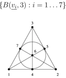
Proof. Consider the incidence matrix of the Fano plane P G(2,2) consisting of 7 rows and columns corresponding to its line and point set, see Figure 1. Let vi be the ith row corre-sponding to theith line in the finite geometry. We show that the following query set provides a separating ball system, implying the lemma:
[image:7.595.251.359.394.522.2]{B(vi,3) :i= 1. . .7}.
Figure 1: Fano plane of order 2
Let u∗ denote the marked element in Q7 and S(u∗) denote the subset of the set of balls
{B(vi,3) : i = 1. . .7} for which u∗ ∈ B(vi,3). We show that any subset S is squarely determined by the choice of u∗. To this end, we study the connection between the support of u∗ and the cardinality of S(u∗).
Observation 2.2. .
(0) |supp(u∗)|= 0 → |S(u∗)|= 7.
(1) |supp(u∗)|= 1 → |S(u∗)|= 3, and S(u∗) consists of the balls, whose centers’ support
contains supp(u∗).
(2) |supp(u∗)|= 2 → |S(u∗)|= 5, and S(u∗) consists of the balls, whose centers’ support
intersects supp(u∗).
(3) |supp(u∗)| = 3 and supp(u∗) corresponds to a line in the Fano plane, i.e. u∗ = vj
(3’) |supp(u∗)| = 3 and supp(u∗) does not correspond to any line in the Fano plane, → |S(u∗)| = 3 and S(u∗) consists of the balls, whose centers’ support intersection with
supp(u∗) has cardinality 2. (Hence, the intersection of the supports of all these 3 centers is the empty set.)
Claim 2.3. S(u∗) ˙S
S(u∗) = {B(v
i,3) : i= 1. . .7}.
Proof. d(u, v) +d(u, v) = 7 for all u, v ∈Q7, thus exactly one of the summands is less then or equal to 3.
Corollary 2.4. |supp(u∗)|>3→ |S(u)| is even.
To complete the proof of Lemma 2.1, it is enough to verify that no set S ⊆ {B(vi,3) :
i = 1. . .7} , |S| odd, is assigned to different elements of Q7. Indeed, the other case S ⊆
{B(vi,3) : i= 1. . .7},|S|even will follow from this in view of Claim 2.3, sinceS(u∗) =S(u0) is equivalent to S(u∗) = S(u0), where |S(u∗)|= 7− |S(u∗)| is odd if |S(u∗)| is even.
But this verification is straightforward according to the case analysis of Observation 2.2, as it is easy to see how the sets S ⊆ {B(vi,3) : i = 1. . .7} are determined accordingly in the cases |S|= 1,3,5 and 7.
3
The Erd˝
os-R´
enyi random graph
In this section we consider the Erd˝os-R´enyi random graphG(n, p). ByG(n, p) we mean the probability space of all labeled graphs onn vertices, where every edge appears randomly and independently with probabilityp=p(n). We say thatG(n, p) possesses a propertyP asymp-totically almost surely, or a.a.s. for brevity, if the probability thatG(n, p) satisfiesP tends to 1 asntends to infinity. We will find bounds for the quantitiesM(G(n, p), r),M(G(n, p),≤r), and M(G(n, p)) which hold asymptotically almost surely. All our searches will use balls of equal radius, so the bounds we find for M(G(n, p),≤r) will hold for M(G(n, p), r) as well.
Before we start to investigate the parameterM(G(n, p),≤r) generally, let us consider the special case when r= 1. In this case the asymptotics of M(G(n, p),≤r) follow immediately from a result of Frieze, Martin, Moncel, Ruszink´o, and Smyth [10]. As we mentioned in the introduction, for any graphGwe always haveM(G,1)≤i(1)1 (G). The parameteri(1)1 (G(n, p)) was studied by Frieze, Martin, Moncel, Ruszink´o, and Smyth who proved the following theorem.
Theorem 3.1 (Frieze, Martin, Moncel, Ruszink´o, Smyth [10]). Let q = p2 + (1−p)2 and
assume p,1−p≥ log loglognn. Then asymptotically almost surely i1(1)(G(n, p)) = (1 +o(1))log(12 log/qn)
holds.
identifying code C of size (2log(1−ε) log/q)n by considering the probability that there exists a pair of vertices inV(G(n, p))\C that is not separated by the closed neighborhoods (i.e. 1-balls) of vertices of C. Since the probability that a setB1 of 1-balls and a setB0 of 0-balls together form a separating system is not larger than the probability that the closed neighborhoods of the centers C of the balls in B1 ∪B0 separate all pairs of vertices in V(G(n, p))\C, we obtain the following corollary of Theorem 3.1.
Corollary 3.2. Let q = p2+ (1−p)2 and assume p,1−p ≥ log loglognn. Then almost surely
M(G(n, p),1) = (1 +o(1))log(12 log/qn) holds.
Let us now consider the problem for general r. Note that all our constructions use balls of equal radius thus all our bounds will apply to i(1)r (G(n, p)) as well. To obtain our bounds on M(G(n, p),≤ r) and M(G(n, p)) we will need two tools. The first tool is the following theorem of Katona.
Theorem 3.3(Katona [15]). LetX be anM-element set andA ⊆2X be a separating system
of subsets of X such that for all A∈ A we have |A| ≤m for some integer m < M/2. Then the following inequality holds
|A| ≥ M
m
logM
logeMm .
Secondly, we will apply the Chernoff inequalities (see [1]).
Chernoff bound: If X is a binomially distributed random variable with parameters n and
p and λ=np, then for any t≥0 we have
P(X ≥EX+t)≤exp
− t
2
2(λ+t/3)
and
P(X ≤EX−t)≤exp
−t
2
2λ
.
Our strategy will be quite simple. Whenever we are allowed to use balls of radius at most
r, we will indeed use balls of radius r and place the centers of the balls randomly. Then we have to analyze how many randomly placed balls will guarantee the separation of all pairs of vertices. Note that in any graphGtwo verticesx, y ∈V(G) are separated by a ball of radius
r with center z∈V(G) if and only ifz ∈BG(x, r)4BG(y, r), where X4Y =X\Y ∪Y \X for any two setsX and Y. Therefore to obtain our results we will need bounds on|B(x, r)|, the sizes of all balls of radius r in G(n, p) and also on the sizes of pairwise intersections of balls of radius r in G(n, p).
Theorem 3.4 (Bollob´as, [3]). (i) Suppose p2n−2 logn → ∞ and n2(1−p) → ∞. Then
G(n, p) has diameter 2 asymptotically almost surely.
(ii) Suppose the functions d = d(n) ≥ 3 and 0 < p = p(n) < 1 satisfy (logn)/d−
3 log logn → ∞, pdnd−1 −2 logn → ∞ and pd−1nd−2 −2 logn → −∞. Then G(n, p) has
diameter d asymptotically almost surely.
Actually, Bollob´as proved more: he showed that ifpdnd−1 = log(n2/c) for some positive constant c, then the distribution of the number of pairs of vertices in G(n, p) that are of distanced+ 1 from each other tends to a Poisson distribution and therefore the probability that G(n, p) has diameter d tends to e−c/2 while the probability that the diameter is d+ 1 tends to 1−e−c/2.
The main lemma which essentially deals with the required bounds on |BG(n,p)(x, r)| and
|BG(n,p)(x, r)4BG(n,p)(y, r)| is Lemma 5 in the paper of Bollob´as. He carries out all calcu-lations only for pdnd−1 = log(n2/c), but when p is bounded away from this threshold value, all calculations are even easier. Let us summarize how Bollob´as obtains his bounds. For a fixed vertex x, we writeB(x, j) = BG(n,p)(x, j) and S(x, j) =B(x, j)\B(x, j−1).
• To obtain bounds on the size ofB(x, r) for a fixed vertexxofG(n, p) Bollob´as exposes the edges of G(n, p) in rounds. In thejth round he exposes edges between S(x, j−1) and V(G(n, p))\B(x, j −1) to determine S(x, j) and thus B(x, j). Note that if we condition on B(x, j−1), then the size of S(x, j) is a binomial random variable as for each vertexyofV(G(n, p))\B(x, j−1) the probability ofy∈S(x, j) is 1−(1−p)|S(x,j)| and these events are independent. Careful analysis of concentration inequalities for binomial random variables gives a very small error probability of|B(x, r)|not behaving as expected. Then the union bound is used to get the result below for all vertices.
• Similarly to the steps above, fixing two vertices x, y of G(n, p) one can expose the edges in the following rounds. In round j one exposes edges between S(x, j−1) and
V(G(n, p))\B(x, j−1) and also betweenS(y, j−1) andV(G(n, p))\B(y, j−1). Vertices inB(x, j)∩B(y, j)\(B(x, j−1)∩B(y, j−1)) may come either fromB(x, j−1)\B(y, j−1) orB(y, j −1)\B(x, j−1) or from V(G(n, p))\(B(x, j −1)∪B(y, j−1)). Thus the number of new vertices in the intersection will be the sum of 3 binomially distributed random variable. Concentration inequalities and the union bound is used again to obtain bounds for all pairs x, y.
Lemma 3.5 (Bollob´as, Lemma 5 in [3]). Let d denote the diameter of G(n, p) with 2 ≤ d
and (logn)/d−3 log logn→ ∞. Then the following holds for G(n, p) asymptotically almost surely: for any 1≤j ≤d−2 and any pair x, y of vertices we have
|BG(n,p)(x, j)|= (1 +o(1))(np)j and |BG(n,p)(x, j)∩BG(n,p)(y, j)|=O(n2j−1p2j).
Lemma 3.5 enables us to obtain bounds on M(G(n, p), r) whenr≤d−2.
Theorem 3.6. Suppose the functions d=d(n)≥3 and 0< p =p(n)<1 satisfy
Then for any 1≤r≤d−2 we have that
(1−o(1))n1−rp−r logn
log(n1−rp−r) ≤M(G(n, p),≤r)≤(1 +o(1))n 1−r
p−rlnn
holds asymptotically almost surely.
Proof. To obtain the lower bound we have to plug the valuesM =nandm= (1 +o(1))(np)r into Theorem 3.3. Note that the value of m follows from Lemma 3.5. Then Theorem 3.3 yields
M(G(n, p), r)≥ logn
loge(1+o(1))(n np)r
n
(1 +o(1))(np)r = (1−o(1))n 1−r
p−r logn
log(n1−rp−r).
To obtain the upper bound we will place balls of radius r at centers u1, u2, ..., ut ∈
V(G(n, p)) chosen uniformly at random and independently of each other. We introduce the random indicator variablesYvi,vj of the event that the verticesvi, vj are not separated by the balls BG(n,p)(u1, r), . . . , BG(n,p)(ut, r). We write Y =
P
1≤i<j≤nYvi,vj to denote the random variable of the total number of unseparated vertices. Observe that by Lemma 3.5 we have
|BG(n,p)(vi, r)\BG(n,p)(vj, r)|= (1 +o(1))(np)r and thus
E(Yvi,vj) =
1−|BG(n,p)(vi, r)4BG(n,p)(vj, r)| n
t =
1− (2 +o(1))(np)
r
n
t
.
Therefore if t≥n1−rp−rlnn holds, then we have
E(Y)≤
n
2 1−
(2 +o(1))(np)r
n
t
≤ 1
2exp(2 lnn−2tn r−1
pr)≤ 1
2.
Therefore there exists a particular choice of u1, u2, ..., ut such that the number of non-separated pairs of vertices is 0.
One would expect that|BG(n,p)(x, d−1)|= (1+o(1))(pn)d−1 should hold. It does for most values ofp, but for a tiny range it fails since ifn−(d−2)/(d−1) ≤p≤n−(d−2)/(d−1)(2 logn)1/(d−1), then (pn)d−1 is larger than n and still the diameter of G(n, p) is d. For this range of p we introduce the function f(n) = fd(n) defined by the equation (np)d−1 = n·f(n). We will subdivide the interval ofp for which the diameter of G(n, p) is d into four smaller intervals. When f(n) → ∞, then balls of radius d−1 consist of almost all vertices, and therefore we will be interested in their complement and in the fact that whether these complements are still bigger than the balls of radiusd−2. If this is so, then it is still worth picking randomly centered balls of radius d−1, than those of radius d−2.
Lemma 3.7. (i) If (np)d−1 =o(n), then a.a.s
|B(x, d−1)|= (1 +o(1))(np)d−1,|B(x1, d−1)4B(x2, d−1)|= (2 +o(1))(np)d−1
(ii) If (np)d−1 = (c+o(1))n holds for some positive constant c, then a.a.s.
|B(x, d−1)|= (1−e−c+o(1))n,|B(x1, d−1)4B(x2, d−1)|= (1−e−2c+o(1))n/ef(n)
hold for all vertices x, x1, x2 ∈V(G(n, p)).
(iii) If f(n)≤(1−ε)d−11logn holds, then a.a.s.
|B(x, d−1)|= (1 +o(1))n/ef(n),|B(x1, d−1)4B(x2, d−1)|= (2 +o(1))n/ef(n)
hold for all vertices x, x1, x2 ∈V(G(n, p)).
(iv) If f(n)≥(1 +ε)d−11logn holds, then a.a.s. we have
|B(x, d−1)|<|B(x, d−2)|
for all x∈V(G(n, p).
Proof. Let us condition on the event that is stated in Lemma 3.5. More precisely, when proving statements about B(x, d−1), we pick a vertex x, expose edges in rounds among verticesS(x, j−1) andV(G(n, p))\B(x, j−1). We condition on the eventEx that|S(x, d− 2)|= (1+o(1))(np)d−2. Bollob´as proved thatE
xholds with probability 1−n−K for some large constantK and thus Ex holds with high probability for all vertices simultanously. Similarly, when proving statements on|B(x1, d−1)∩B(x2, d−1)|we pick two verticesx1andx2, expose edges in rounds among vertices inS(x1, j−1) and V(G(n, p))\B(x1, j−1) and also among vertices inS(x2, j−1) and V(G(n, p))\B(x2, j−1). We condition on the eventEx1,x2 that
|S(x1, d−2)|= (1+o(1))(np)d−2 =|S(x2, d−2)|and|B(x1, d−2)∩B(x2, d−2)|=O((np)d−3). Again, these events hold with probability 1−n−K for some large constant K.
Before considering the four cases let us observe that Ω(n1/2) = (np)d−2 =o(n). We will also use the inequalities pa−p2 a
2
≤1−(1−p)a≤pa.
Consider first the cases (i), (ii) when (np)d−1 =o(n) or (np)d−1 = (c+o(1))n holds for some positive constantc. In this case for a vertexy /∈B(x, d−2) we haveP(y∈S(x, d−1)) = 1−(1−p)|S(x,d−2)|. This is (1 +o(1))pd−1nd−2 and thus
E(|S(x, d−1)|) = (1 +o(1))(np)d−1 if (np)d−1 = o(n), while (n −o(n))(1−(1−p)|S(x,d−2)|) = (1−e−c+o(1))n if (np)d−1 = (c+o(1))n. As (np)d−1 ≥(np)d−2 = Ω(n1/2) holds, by Chernoff’s inequality we obtain that P(|S(x, d−1)−E(|S(x, d−1)|)| ≥n1/3) is exponentially small in a positive power of n. The union bound gives that asymptotically almost surely|B(x, d−1)|= (1 +o(1))|S(x, d−1)|= E(|S(x, d−1)|) holds for all vertices.
Let us condition on the sets B(x1, d−2), S(x1, d−2), B(x2, d−2) andS(x2, d−2). Then a vertex y can become an element ofB(x1, d−1)∩B(x2, d−1) in the following ways:
(a) eithery /∈B(x1, d−2)∪B(x2, d−2) and (a1) it is connected to a vertex inB(x1, d− 2)∩B(x2, d −2) or (a2) is connected to at least one vertex both from S(x1, d−2) and
S(x2, d−2) or
(b) y∈ S(x1, d−2)\B(x2, d−2) and y is connected to a vertex in S(x2, d−2) or vice versa. The number of such vertices is binomially distributed in all three cases.
In case (a1), using the result of Lemma 3.5 on |B(x1, d −2) ∩B(x2, d − 2)| the ex-pected value of such vertices isO(p2(d−2)+1n2(d−2)) =O((pnp)2((pn)
d−1)2) = O( pn (pn)2(pn)
d−1) =
In case (a2), the expected value of such vertices is (1−(1−p)|S(x1,d−2)|)(1−(1−p)|S(x2,d−2)|) which is O(n1((pn)d−1)2) = o((pn)d−1) provided (np)d−1 = o(n). If (np)d−1 = (c+o(1))n, then this value is (1−e−c)2+o(1)n.
Finally, in case (b), the expected value of such vertices isO((pn)d−2pd−1nd−2) =o((pn)d−1). In all three cases Chernoff’s inequality and the union bound can be applied to obtain the same bounds not only for one, but all pairs of vertices.
Altogether, we obtain that |B(x1, d−1)4B(x2, d−1)|= (2 +o(1))(np)d−1 holds almost surely for all x1, x2 if (np)d−1 = o(n) and that |B(x1, d−1)4B(x2, d−1)| = [2(1−e−c)− (1−e−c)2+o(1)]n = (1−e−2c+o(1))n if (np)d−1 = (c+o(1))n holds.
Let us now turn our attention to (iii) and (iv). In these cases we are interested in
|B(x, d−1)|. Let us repeat that f(n) is defined by f(n) = fd(n) = (np)d−1 = n ·f(n) and that f(n) tends to infinity as otherwise we were in case (i) or (ii). If we condition on B(x, d−2) and S(x, d−2), then the size of B(x, d−1) is binomially distributed with E(|B(x, d−1)|) = (n− |B(x, d−2)|)(1−p)|S(x,d−2)|= (1 +o(1))elogn−(1+o(1))f(n). If f(n)≥ (1 +ε)d−11 logn holds for some positive ε, then this expression is o((np)d−2). Chernoff’s inequality and the union bound ensures that this holds for all x and we are done by (iv).
Using Chernoff’s inequality we obtain that as long as f(n) ≤ (1−ε)d−11logn holds, we have a.a.s |B(x, d−1)| = (1 + o(1))n/ef(n) > |B(x, d − 2)| for any vertex x. As
I := B(x1, d−1) ∩B(x2, d−1) = B(x1, d−1)∪B(x2, d−1) we have that for any y ∈
V(G(n, p))\(B(x1, d−2)∪B(x2, d−2)) the probability thatyis inIis (1−p)|S(x1,d−2)∪S(x2,d−2)| and thusE(|I|) = (1 +o(1))n/e2f(n). Note that as f(n) tends to infinity, we haven/e2f(n)=
o(n/ef(n)). The usual Chernoff’s inequality argument shows that|B(x1, d−1)∩B(x2, d−1)|=
o(n/ef(n)) and thus |B(x
1, d−1)4B(x2, d−1)| = (2 + o(1))n/ef(n) holds a.a.s for any
x1, x2 ∈V(G(n, p)).
The results of Lemma 3.7 enable us to imitate the proof of Theorem 3.6 to obtain bounds on M(G(n, p)). Part (iv) of Lemma 3.7 shows that in that range of p, one cannot improve the bounds of Theorem 3.6 by using random balls of radiusd−1. In all other cases, replacing the values of |B(x1, d−1)4B(x2, d−1)|=|B(x1, d−1)4B(x2, d−1)|does indeed improve on bounds obtained by placing balls of radius d−2. However, their formulation would be a little lengthy due to the fact that sometimes one has to calculate with the size of balls of radius d−1 and sometimes with the size of their complements. Therefore here we state only the simplest case (corresponding to case (i) in Lemma 1.7.) and just mention that in all cases the lower and upper bounds that can be obtained differ only by a factor of a power of logn.
Theorem 3.8. Suppose the functionsd=d(n)>3and0< p=p(n)<1 satisfy(logn)/d−
3 log logn → ∞, pdnd−1−2 logn→ ∞. Furthermore, if (np)d−1 =o(n)holds, then a.a.s we
have
(1−o(1)) n (np)d−1
logn
logn/(np)d−1 ≤M(G(n, p))≤(1 +o(1))
n
4
Graphs of bounded maximum degree
The aim of this section is to prove Theorem 1.2, that is for any G ∈ G∆,n we have A(G) = Θ∆(logn) where G∆,n denotes the set of finite graphs on n vertices with maximum degree at most ∆. Note that the lower bound logn ≤ A(G) holds for any graph as the sequence of answers must differ for all vertices of G. The idea behind Theorem 1.2 is the following: for every G ∈ G∆, v ∈ V and r ≥ 1 we have |BG(v, r + 1)|/|BG(v, r)| ≤ ∆−1, and this enables us to imitate the halving argument of adaptive binary search. This is formulated in the following lemma.
Lemma 4.1. Let G be a connected graph with maximum degree ∆. For every X ⊆ V(G)
with |X| ≥∆ + 2, there exists a vertex v(X)∈V(G) and a natural number r(X) satisfying
1
∆ + 2|X| ≤ |B(v(X), r(X))∩X| ≤
∆ + 1 ∆ + 2|X|.
Proof. For all w∈V(G) andX ⊆V(G) we define the following function:
f(w, X) := min
r:|B(w, r)∩X| ≥ ∆ + 1
∆ + 2|X|
.
Since G is connected, f(w, X) is well defined for all w ∈ V(G). Also observe that
f(w, X)≥2, since ∆+1∆+2|X| ≥∆ + 1.
Define m(X) = min{f(w, X) : w ∈ V(G)}, and let w(X) be any vertex satisfying
f(w(X), X) = m(X). We claim that we can choose one of the neighbours of w(X) as our vertexv(X). Suppose, for the sake of contradiction, that none of the neighbors ofw(X) fulfill the statement of the lemma. By the definition ofm(X), we know that|B(u, m(X)−1)∩X| ≤
1
∆+2|X| holds for all vertices u∈V(G). But we also know that
B(w(X), m(X))⊆ [
{u,w(X)}∈E(G)
B(u, m(X)−1).
This gives us
X∩B(w(X), m(X)) ⊆ X∩ [
{u,w(X)}∈E(G)
B(u, m(X)−1).
This gives a contradiction since |X∩B(w(X), m(X))| ≥ ∆+1
∆+2|X| holds by the definition of
m(X), whereas |X ∩S
{u,w(X)}∈E(G)B(u, m(X)−1)| ≤ P
{u,w(X)}∈E(G)|B(u, m(X)−1)| ≤ ∆
∆+2|X|.
Now we are ready to prove Theorem 1.2.
Proof of Theorem 1.2: Let G ∈ G∆,n be a connected graph and set X0 = V(G). For i > 0 we repeatedly apply Lemma 4.1 to Xi−1 as long as |Xi−1| ≥∆ + 2 holds. We ask the query
Xi := (
Xi−1∩B(v(Xi−1), r(Xi−1)) if the answer is yes;
Xi−1\B(v(Xi−1), r(Xi−1)) if the answer is no.
Clearly the unknown vertex is contained in Xi for all values ofi. If |Xi−1| ≤∆ + 2, then we ask its vertices one by one (more precisely the balls of radius 0 around its vertices). The length of this process is at most
log∆+3
∆+2n+ ∆ + 1. This completes the proof of the theorem.
By the same argument, one can prove a version of Theorem 1.2 where the upper bound ∆(n) on the maximum degree in the graph is a function which grows with n. Namely, we obtain a log∆(n)+3
∆(n)+2
n+ ∆(n) + 2 upper bound on the length of an adaptive search.
References
[1] N. Alon and J. Spencer. The probabilistic method. Wiley-Interscience., 1991.
[2] Y. Ben-Haima, S. Gravierb, A. Lobsteinc, and J. Moncel. Adaptive identification in graphs. J. Combin. Theory Ser. A, 115(7):1114–1126, 2008.
[3] B. Bollob´as. The diameter of random graphs. Trans. Amer. Math. Soc., 267:41–52, 1981.
[4] I. Charon, G. Cohen, O. Hudry, and A. Lobstein. New identifying codes in the binary hamming space. European J. Combin., 31:491–501, 2010.
[5] G. Cohen, I. Honkala, S. Litsyn, and A. Lobstein. Covering Codes. North-Holland Publishing Co., 1997.
[6] G. Exoo, V. Junnila, T. Laihonen, and S. Ranto. Upper bounds for binary identifying codes. Advances in Applied Mathematics, 42(3):277–289, 2009.
[7] G. Exoo, V. Junnila, T. Laihonen, and S. Ranto. Improved bounds on identifying codes in binary Hamming spaces. European J. Combin., 31(3):813–827, 2010.
[8] G. Exoo, T. Laihonen, and S. Ranto. New bounds on binary identifying codes. Discrete Applied Mathematics, 156(12):2250–2263, 2008.
[9] F. Foucaud and G. Perarnau. Bounds for identifying codes in terms of degree parame-ters. Electron. J. Combin., 19, 2012.
[10] A. Frieze, R. Martin, J. Moncel, M. Ruszink´o, and C.Smyth. Codes identifying sets of vertices in random networks. Discrete Math., 307:1094–1107, 2007.
[12] S. Janson and T. Laihonen. On the size of identifying codes in binary hypercubes. J. Combin. Theory Ser. A, 116(5):1087–1096, 2009.
[13] V. Junnila. Adaptive identication of sets of vertices in graphs. Discrete Math. Theor. Comput. Sci., 14(1):69–86, 2012.
[14] M. G. Karpovsky, K. Chakrabarty, and L. B. Levitin. On a new class of codes for identifying vertices in graphs. IEEE Trans. Inform. Theory, 44:599–611, 1998.
[15] G. Katona. On separating systems of a finite set. J. Combin. Theory, 1(2):174–194, 1966.
[16] G. Katona. Combinatorial search problems, problem booklet of the 5th eml´ekt´abla workshop, http://www.renyi.hu/∼emlektab/index−booklet.html. 2013.
[17] V. L. Klee and D. G. Larmann. Diameters of random graphs. Canad. J. Math., 33:618– 640, 1981.
[18] M. Krivelevich, B. Sudakov, and V. H. Vu. Covering codes with improved density. IEEE Trans. Inform. Theory, 49:1812–1815, 2003.
[19] A. Lobstein. http://www.infres.enst.fr/∼ lobstein/debutbibidetlocdom.pdf.
[20] J. Moncel. Codes identifiants dans les graphes. These de Doctorat, Universit´e de Greno-ble, France, 2005.