Predictions vs preliminary sample estimates

Munich Personal RePEc Archive

Predictions vs preliminary sample

estimates

D’Elia, Enrico

ISAE (Institute for studies and economic analisys) Rome (Italy)

2010

Online at

https://mpra.ub.uni-muenchen.de/36070/

Predictions

vs

preliminary sample estimates

Enrico D’Elia (Isae) [email protected]

ABSTRACT

In general, rational economic agents are not in the position to wait for the statistical agencies disseminate the final results of the relevant surveys before making a decision, and have to make use of some model based predictions, even when agents are not assumedly forward looking. Thus, from the viewpoint of agents, predictions and preliminary results from surveys often compete against each other. Agents are aware to incur in a loss basing their decisions on predictions instead of sound statistical data, but the loss could be smaller than the one related to waiting for the dissemination of final data. Comparing the loss attached to predictions, on the one hand, and to possible preliminary estimate from incomplete samples, on the other, provides a broad guidance in deciding if and when statistical agencies should release preliminary and final estimates of the key variables. The main result of the analysis is that, in general, preliminary sample estimates are useful for the users only if they come from unexpectedly large sub-samples, even when the predictability of relevant variables is scarce. Nevertheless, the cost of delaying decisions for many economic agents may support the dissemination of early estimates of the main economic aggregates even if their accuracy is not fully satisfactory from a strict statistical viewpoint.

KEYWORDS: Accuracy, Data Dissemination, Forecast, Preliminary Estimates, Timeliness. J.E.L. CLASSIFICATION: C44, C49, C82, C83.

TABLE OF CONTENTS

1 Introduction 1

2 Comparing the accuracy of preliminary sample estimates and forecasts 2

3 The cost of delaying decisions 6

4 Conclusive remarks 8

References 10

Better to light one candle than to curse the darkness Procrastination is the thief of time

Old English sayings

1 Introduction (*)

Rational economic agents base their decisions partly on statistical data describing the current state of the word. Nevertheless, even when they are not assumedly forward looking, generally are not in the position to wait for the dissemination of the final results of the relevant surveys before making a decision. In fact, timing matters in many decision processes, such as investment, consumption, coordination between supply and demand of non storable goods and services, choice between leisure and working time, etc.Thus, the users of statistical data often have to make some model based predictions about the outcome of statistical surveys, usually referred to as “nowcasts”. As a consequence, from the viewpoint of agents, predictions and preliminary results from surveys often compete against each other. This fact adds new elements to the long lasting debate on the trade off between timeliness and accuracy of official statistics.

Recently, this issue has been addressed mainly with reference to “flash” estimates of GDP and other

“Principal European Economic Indicators” pointed out by the Economic and Financial Committee of the European Commission, and aimed at detecting earlier the turning points of the business cycle.

1

Also OECD analyses the trade-off between accuracy and timeliness of statistical information

within the “Short-Term Economic Statistics Timeliness Framework”. 2 Indeed, the official statistical agencies have made a remarkable effort in providing the users with early model based estimates of the main economic aggregates. 3 In fact, the European Central Bank (2009) remarked even recently that the flash estimate of GDP do not differ significantly from that provided by the first full release published later, which means that they are likely more helpful for the decision makers than the corresponding final releases. 4

At time t+h, the predictions on the status of the relevant variables at time t can be based only on an information set, say t+h, smaller than the one possibly available by the end of the relevant surveys,

at time t+H. Agents are aware to incur in a loss, say F(h), if they make decision at time t+h instead

(*) _{The views expressed in the paper are those of the author and do not necessarily reflect views at ISAE. The author}

gratefully acknowledges the valuable suggestions and criticisms come from some early readers of the paper. Of course, errors or omissions are the responsibility of the author.

1 _{Recently, the topic has been discussed in depth in an international conference organised by UNSTATS (2009).} 2 _{Related documents are available at www.oecd.org/document/40/0,3343,en_2649_34257_30460520_1_1_1_1,00.html.}

3 _{See Bruneau et al. (2007) and Duarte and Rua (2007) for some nowcasting models of inflation; Bruno and Lupi (2004)}

about the flash estimates of the industrial production index; Giannone, Reichlin and Small (2008) about joint nowcast and short term forecast of inflation and GDP; Altissimo et al. (2007), Frale et al. (2007) and Diron (2008) for the use of the so-called bridge equations in nowcasting and predicting GDP; Pain and Sédillot (2005), Angelini et al. (2008) and Barhoumi et al. (2008) about very short term forecast and nowcast of GDP.

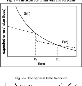
of waiting until t+H. Assuming that news prevail on noise, 5 the accuracy of nowcast likely improves as time goes on, so that F(h) decreases with h. On the other hand, collecting and elaborating data within a statistical survey takes time, thus the expected accuracy of possible preliminary sample estimates increases as data accumulate. As a consequence, the loss associated to the use of preliminary estimates based on the information set including only the data collected until t+h, is a decreasing function of h as well, say S(h). However, at time t+H, after data collection and elaboration has been completed, surveys hopefully provide results much more accurate than the best forecasts. Thus the advantage of using forecast, say F(h) – S(h), turns out to be a decreasing function of h as well.

As long as the statistics should meet users’ needs, the comparison between F(h) and S(h) provides a broad guidance in deciding when and how preliminary and final estimates should be released. In fact, users would take advantage from the dissemination of preliminary data only if they provide better information compared to available forecasts, that is as far as S(h) < F(h), otherwise they would continue using their forecasts.

The main aim of this paper is to study the consequences of the availability and reliability of model based forecasts in devising the optimal dissemination policy of the statistical agencies. The next section reports some well known properties of the preliminary estimates from incomplete samples and derives an optimal calendar for disseminating preliminary estimates comparing their accuracy to the errors size of model based predictions. The third section introduces the topic of the cost of delaying decisions waiting for better sample estimates. Some conclusive remarks close the paper.

2 Comparing the accuracy of preliminary sample estimates and forecasts

Let xi,t be a quantitative character, with average mt, measured on the i-th individual, and related to

its status at time t. At time t+h users can obtain at least two provisional estimates of the variable of interest mt: the first one, say st+h, is the preliminary estimate based on the incomplete sample of the

first M data collected; the other, say ft+h = E(mt|t+h), is the forecast produced by a model which

exploits the information set t+h that assumedly excludes the results of the latter survey.

If the survey is repeated regularly over time, the time series {xi,t} can be decomposed as

xi,t = ft+h + vt+h + ei,t [1]

3 where vt+h = mt  ft+h is an innovation process, such that E(vt+h|t+h) = 0 and E(vt+h2|t+h) = _h2,

under the assumption that, on average, the accuracy of forecast does not depend on t;6 ei,t is a

random individual component, with E(ei,t) = 0 and E(ei,t2) = 2. Since t+h t+h-1 by definition, it

follows that

dh d_h

≤ 0.

Let’s suppose, without any loss of generality, that the index i denotes the collection order of data, then the preliminary estimates st+h is

st+h =





h t

M

i 1

wi,t,h xi,t [2]

where Mt+h is the number of data collected at time t+h, and the weights wi,t,h sum to one. If data

pour in randomly, subsamples of data available in each moment are assumedly unbiased, thus the average of st+h (evaluated for all the possible samples of size Mt+h) is E(st+h) = mt. Furthermore, if

the individual deviations from the general average are mutually independent, the usual assumption E(eiej) = 0, for i≠j applies, so that the variance of st+h is

h =





h t

M

i

h , t , i

w 1

2



[3]

which in the simplest case of equally weighted observations reads

h =

h t

M _



[4]

Of course, h is infinite before the survey begins, since then Mt+h is null. In any case, Mt+h is a non

decreasing function of h, say Mt+h = M(h) with dh dM

> 0, regardless to the reference period t. It

follows that

dh d _h

< 0. Furthermore,

2 2

dh d  _h

< 0 in the most favourable case in which “better”

data are collected by the beginning of the survey process and the data collection proceeds until the

6 _{The latter condition is violated when some time specific factor changes systematically the predictability of the relevant}

informative contribution of any further observation is negligible. 7 Thus, if the loss function S(h) is a monotonically increasing function of h, say S(h) = L(h) with

h

d dL

 > 0, [4] implies that S(h) decreases with h at a decreasing rate as well, under fairly general conditions. 8

In the simplest case [4], the decomposition [1] implies that

E( _H2 ) =





        



M x f

E

1

2

1 _{ 2}

h

 [5]

where the E(.) operator applies to the time series of the relevant variables and the parameters  2_H and _h2 are possibly time varying. The expression in square brackets in [5] is larger than  _H2 , since only the arithmetic average mt minimizes the sum of squared discrepancies





thus _h2 can be seen as the difference between the estimated variance among observations around the forecast ft+h, on the one side, and the variance  _H2 around the true average mt, on the other.

Thus _h2 is likely small compared to  _H2 , as long as ft+h is a quite reliable forecast of mt, on

average.

Rational agents are assumedly able to make some forecast even before data collection has begun, so that the accuracy of their initial predictions is always better than every preliminary estimate based on collected data. Later, predictions may improve, thanks to the possible availability of other relevant information, but likely at a slower pace, compared to any survey. Otherwise, forecast beat statistical surveys all the time, and paradoxically the latter would be useless at all.

The assumptions that F(0) < S(0) but

dh dS

≤ dF_dh ≤ 0 imply that F(h) = S(h) at some point in time, 9 say t+h0. In particular, rational agents would use preliminary results of statistical surveys only if

7 _{In fact, the assumptions on M(h) imply that}

dh d _h

= 3 2 M   dh dM

< 0. Furthermore, it reads

2 2

dh d  _h

= 3 2 M                 2 2 2 2 3 dh M d M dh dM

, whose sign depends on the sign of the expression within the square

brackets. In particular, if the data collection process is concentrated by the beginning of the survey, as assumed above,

2 2

dh M d

< 0, so that

2 2

dh d  _h

> 0.

8 _{The main limitation of assuming}

h

d dL

 > 0 is that positive forecast errors imply the same loss of negative ones. See

5 they are published later than t+h0. However, if the statistical agencies actually decide to release the

estimates at time t+h0 the information set used to make forecasts also improve, thus the expected

error size of predictions falls as in Fig. 1. The improvement is null if the statistical agencies provide

the best nowcast by applying some model based estimator to the collected data, so that the users’

forecast could hardly beat the preliminary estimates published at time t+h. 10

[insert Figure 1 about here]

Nevertheless, if the users have got some private information about mt, or the statistical agencies are

unwilling to publish model based estimates, every publication of preliminary estimates from a sub sample induces a further downward shift in the function F(h), determining a new crossing points between F(h) and S(h), say at the delay h1, and so on. Thus, an optimal schedule for the

dissemination of preliminary and final estimates can be defined.

Of course, the sequence of data publication depends heavily on the process of data collection and elaboration of data and on their predictability. Furthermore, the dissemination of preliminary and final results of surveys beyond (before than) the ones suggested by the comparison between F(h) and S(h) is not fully worthless as long as that results improve the information set used to form nowcasts and forecasts as well. In particular, the shape and level of F(h) depends on information available at time t+h, that may or not include preliminary and final data referred to the past.

The relative performance of the two estimators of mt depends on the time schedule of the survey,

which determines the coverage ratio

H t

h t

M M

 

, and on the ratio h =

H h

 

of the mean square error

of prediction to the variance of mt among observations by the end of the survey. The ratio hranges

from 0 to infinity: in particular, h is null if the time series mt is purely deterministic and tends to

infinity if individuals are identical. 11

9 _{The sign of}

2 2

dh d  _h

is not relevant for the functions F(h) and S(h) cross each other.

10 _{The improvement in nowcast can be seen as a special case of exploiting efficiently the data collected up to t+h} 0 by

integrating missing data in the full sample by means of a model based estimator, as discussed in Sarndal (2005). Furthermore, the users can only combine available forecasts, as suggested by Clemen (1989) and Yang and Zou (2004), while the statistical agencies possibly may combine the same forecasts and the provisional results of their surveys.

11 _{For instance, the mean age of a stationary population can be virtually predicted without any error even though the age}

As assumed above cautiously, let the forecast accuracy improve over time less than

H h

 

, that is

less than

h t

H t

M M

 

according to [4]. Since rational agents prefer their own forecast to preliminary

estimates of mt as long as h≥ h, it follows that

H t

h t

M M

  _

h H

 

[6]

The inequality [6] has a number of interesting consequences. First of all, it implies that the sub sample estimator is more efficient after some threshold h only if 0 is not null, otherwise a rational

agent would be always better off by making decisions based on nowcasts. Conversely, the preliminary results from incomplete sample are the best choice at all times only in the limiting case in which even one single observation provides better information than any forecast, so that  is null

for whatever small delay . Secondly, the threshold

H t

h t

M M

 

for making the publication of

preliminary results appealing may be unexpectedly large even when prediction accuracy is quite poor compared to final sample mean variance H. For instance, if 0 is as (implausibly) large as ten

times H, the minimum sub sample for data publication would be larger than 10% of final sample.

3 The cost of delaying decisions

Often, rational agents have to balance the cost of making decisions based on inaccurate data with the cost of delaying decisions. 12 This is typically the case when the “first mover” has some advantage over the followers, as occurs in a competitive environment. For example, if the potential market is given, the first firm entering the market may hopefully serve the most profitable segment of the demand, while the followers have to supply only the others. Also purchasing and investment decisions are usually supposed to have an optimal timing, mainly related to economic fluctuations.13 In some special cases, taking into account also the cost of delaying decisions may imply that users incur in a smaller overall loss if they base their decisions on nowcasts instead of preliminary and final sample estimates of the relevant vaiables. In fact, the loss of delaying decisions may be so fast growing over time that agents cannot afford to wait for even preliminary survey results. Under these

12 _{See Granger and Machina (2006).}

7 circumstances, actual survey results would be possibly embodied only in the forecasts about the future, but not in the decision process determining current actions directly.

The cost of delaying decisions waiting for more accurate information is presumably a function of time passed from the reference period of relevant information, say D(h). The function D(h) achieves its minimum at h=0, when assumedly D(0) = 0 without any loss of generality. Furthermore,

dh dD

> 0

since the cost of delaying decisions likely rises with h. Also

2 2

dh D d

> 0 can be assumed, as the cost

of the delay increases more than proportionally with h, and becomes virtually infinite when relevant information comes too late for whatever decision.

Supposing that the functions F(h) and S(h) cross at the delay hc, rational agents exploiting only

predictions incur in the minimum overall loss Lp at hp, that is approximately

Lf = (F(hc) + D(hc)) + (f’ + d’) (hf hc) + (p” + d”) (hf hc)2 [7]

while those basing their decisions on the preliminary results of surveys face the minimum loss Ls hs

periods after the reference time, that is about

Ls = (S(hc) + D(hc)) + (s’ + d’) (hs hc) + (s” + d”) (hs hc)2 [8]

where x’ =

c h h dh dX 

and x” =

c h h dh X d  2 2 .

According to [7] and [8], the losses Lf and Ls achieve their minima when hf and hs are respectively

hf = hc

" d " f ' d ' f   2 1 [9] and

hs = hc

" d " s ' d ' s   2 1 [10] that is when

Lf = (F(hc) + D(hc))  4 1 " d " f ) ' d ' f (   2 [11] and

the functions S(h), F(h) and D(h). Indeed, since F(hc) = S(hc) by definition, the condition for Lf <

Ls, together with [11] and [12], imply that

" "

) ' '

( 2

d s

d s

 

>

" d " f

) ' d ' f (



 2

[13]

Assuming that forecasts improve over time only very slightly, and much less faster than the results of surveys, it holds f’  0 and s” > f”. Thus [13] also means that

s’ > 2d’ [14]

As a consequence, even under assumptions very unfavourable to the forecasts, agents would be better off basing their decisions on some predictions, instead of waiting for the preliminary and the final results of relevant surveys, if the marginal improvement of survey accuracy, that is s’, does

not exceed twice the loss attached to postponing decisions one unit of time more, that is d’. The condition [14] fully conforms the intuition, according to which agents prefer basing their decisions on predictions as the cost of delay increases very fast, and the expected error size of surveys does not fall too fast over time.

[insert Figure 2 about here]

Of course, condition [14] does not hold necessarily, so that, in general, agents hopefully find less costly to wait for the dissemination of the final or even preliminary results of statistical surveys. Nevertheless, Fig. 2, shows that even a “moderate” loss function related to decision delaying, applied to the accuracy improvement of predictions and surveys assumed in Fig. 1 gives rise to the result foreseen by [14].

It is worth noticing that the result [14] does not take into consideration the possibility that disseminating preliminary survey results might increase the accuracy of forecast dramatically. Otherwise, it could happen that the minimum loss associated to predictions is always lower than that deriving from making decisions based only on survey results, since, in this case, the curve F(t) + D(t) lies below S(t) + D(t) by definition.

4 Conclusive remarks

Regarding the results of statistical surveys as an input for decisions may provide a broad guidance to design an optimal calendar for data release. Under many circumstances, rational agents likely would appreciate less accurate data in advance instead of delayed perfect statistics, and the

9 variables autonomously. Thus, provisional data assumedly improve their decisions only if the accuracy of published data is capable to beat available nowcasts. Otherwise, rational agents would be better off basing their decisions on simple predictions. It follows that the size of forecast errors should be the main benchmark in deciding when and how frequently statistical data can be released. Furthermore, the same criterion may help statisticians to decide the timing for the dissemination of disaggregated data. In fact, agents who need a given break down level of data, e.g. at N “digits” level of the NACE classification of branches of economic activity, to make a decision necessarily compare the loss associated to the use of preliminary survey results at N digit level, say S*(N), to the loss of using some model based estimation which exploits only data already available, e.g. data broken down at N-n digits, say F*(N-n). Thus, at time t+h, statistical data disaggregated at level N would be long-awaited by agents only if F*(N-n) > S*(N), otherwise users would be better off if statistical agencies had released earlier data disaggregated at level N-n instead.

Some back-of-the-envelope reckoning shows that comparing the accuracy of nowcast and preliminary sample estimates gives support for disseminating only the results of unexpectedly large sub-samples. In fact, the inaccuracy of forecast on aggregated data generally confronts large variance of individuals around the average. Of course, statistical agencies would beat any other nowcast if they exploit sample information within the framework of a proper model based estimator. The good practices in early estimates of GDP, adopted by most statistical offices, provide an example of the efficiency gain possibly attained by combining raw preliminary statistical information and econometric methodologies. Another successful example of integrating sample results and econometrics is the release by Eurostat of early estimates of the harmonised index of consumer prices for the European Union and the Eurozone.

Further support for statistical agencies disseminate preliminary results of their surveys comes from the fact that rational agents often balance the cost of making a decision based on inaccurate data with the cost of delaying their decisions. If timing is crucial in making a decision, even very noisy and inaccurate preliminary data would be appreciated under most circumstances.

References

Altavilla, C. and M. Ciccarelli (2007), “Information combination and forecast (st)ability. evidence from vintages of time-series data”, Working Paper Series ECB, No. 864.

Altissimo, F. et al. (2007), “New EUROCOIN: tracking economic growth in real time”, Banca d'Italia, Temi di discussione, No. 631.

Angelini, E., G. Camba-Mendez, D. Giannone, L. Reichlin, and G. Rünstler (2008), “Short-term Forecasts of Euro Area GDP Growth”, ECB Working Paper, No. 949.

Barhoumi, K. et al. (2008), “Short-term forecasting of GDP using large monthly datasets: a pseudo real-time forecast evaluation exercise”, Occasional Paper SeriesECB, No. 84.

Blanchard, O. J., J. P. L'Huillier and G. Lorenzoni (2009), “News, noise, and fluctuations: An empirical exploration”, NBER Working Paper, No. w15015

Bruneau, C., O. de Bandt, A. Flageollet and E. Michaux (2007), “Forecasting inflation using

economic indicators: the case of France”, Journal of Forecasting, Vol. 26, No. 1, pp. 1-22.

Bruno, G. and C. Lupi (2004), “Forecasting industrial production and the early detection of turning points”, Empirical Economics, Vol. 29, No. 3, pp. 647-671.

Clemen, R. (1989), “Combining forecasts: a review and annotated bibliography”, International Journal of Forecasting, Vol. 5, pp. 559-583.

Diron, M. (2008), “Short-term forecasts of euro area real GDP growth: an assessment of real-time performance based on vintage data”, Journal of Forecasting, Vol. 27, pp. 371-390.

Duarte, C. and A. Rua (2007), Forecasting infl ation through a bottom-up approach: How bottom is bottom? Economic Modelling, Vol. 24, pp. 941-953.

European Central Bank (2009), “Revisions to GDP estimates in the euro area”, Monthly Bulletin, No. 4, pp. 85-90.

Frale C. et al. (2007), "A monthly indicator of the Euro area GDP", Working Paper CEPR, No. 7007.

Giannone D., L. Reichlin, D. Small (2008), “Nowcasting: The real-time informational content of macroeconomic data”, Journal of Monetary Economics, Vol. 55, No. 4, pp. 665-676

Granger, C.W.J. and M. J. Machina (2006), “Forecasting and decision theory”, in Elliott, G., C.W.J. Granger and A. Timmermann (eds.), Handbook of Economic Forecasting, Vol. 1,Elsevier.

Granger, C.W.J. and M.H. Pesaran (2000), “Economic and statistical measures of forecast accuracy”. Journal of Forecasting, Vol. 19, pp. 537–560.

Pain, N. and F. Sédillot (2005), “Indicator models of real GDP growth in the major OECD

economies”, OECD Economic Studies, No. 40.

11 UNSTAT (2009), “International seminar on timeliness, methodology and comparability of rapid estimates

of economic trends”, http://unstats.un.org/unsd/nationalaccount/workshops/2009/ottawa.

Winston, G. C. (2008), The timing of economic activities, Cambridge, Cambridge University Press. Yang, Y. and H. Zou (2004), “Combining time series models for forecasting. Inter-national Journal

Fig. 1 – The accuracy of surveys and forecasts

time

e

x

p

e

c

te

d

e

rr

o

rs

'

s

ize

(

lo

s

s

)

h₀ S(h)

F(h)

h₁

Fig. 2 – The optimal time to decide

delay

lo

s

s

S(h) + D(h)

F(h) + D(h)

D(h)