Hidden Markov models with t components Increased persistence and other aspects

Munich Personal RePEc Archive

Hidden Markov models with t

components. Increased persistence and

other aspects

Bulla, Jan

October 2009

Hidden Markov models with

t

components.

Increased persistence and other aspects

Jan Bulla

D´epartement de Math´ematiques

Bd Mar´echal Juin, BP 5186

14032 Caen Cedex, France

Phone: +33 (0) 231 56 73 22, Fax: +33 (0) 231 567320

Email: [email protected]

October 2009

Abstract

Hidden Markov models have been applied in many different fields dur-ing the last decades, includdur-ing econometrics and finance. However, the lion’s share of the investigated models is Markovian mixtures of

Gaussian distributions. We present an extension to conditional t

-distributions, including models with unequal distribution types in dif-ferent states. It is shown that the extended models, on the one hand, reproduce various stylized facts of daily returns better than the com-mon Gaussian model. On the other hand, robustness to outliers and persistence of the visited states increases significantly.

Keywords: Hidden Markov model, Markov-switching model, state

persistence, t-distribution, daily returns.

JEL classification codes: C22, C51, C52, E44.

Acknowledgments: We would like to sincerely thank Prof. T. Ter¨asvirta, Prof. P. Thomson, and Prof. W. Zucchini for their inspiring comments and support, and also render thanks to the

partici-pants of the Cherry Bud Workshop 2007 and the 17th NZESG for helpful feedback. Moreover, we

thank two anonymous referees whose comments led to major improvements of the paper, Dr. I. Bulla,

Dr. S. Mergner, and Dr. K. Thangavelu for editorial assistance, and G. Allardice, W. Allardice, and

Prof. D. Vere-Jones for the great working environment. The work of Jan Bulla was supported in parts

1

Introduction

The hidden Markov model (HMM) was introduced in the late sixties (Baum & Petrie 1966, Baum et al. 1970) and since then applied in many fields, such as biology (Koski 2001, Durbin et al. 1998), environmental time series (MacDonald & Zucchini 1997), and speech recognition (Rabiner 1989). Ap-plications related to financial econometrics followed mainly after the seminal works of Hamilton (1989, 1990) on Markov-switching models (a synonym for the HMM).

Amongst the early articles in finance is also Turner et al. (1989), who first considered a Markov mixture of normal distributions to model return series. The presumably best-known article on daily return series and the HMM is authored by Ryd´en et al. (1998), who showed that a Markovian mixture of normal variables reproduces most of the stylized facts for daily return series introduced by Granger & Ding (1995a,b). Other works followed (e.g., Linne 2002, Bialkowski 2003). However, as in many other applications the hidden Markov models (HMMs) considered mainly focus on mixtures of Gaussian distributions.

In this paper, we present an extension of the HMM by replacing the con-ditional Gaussian distribution stepwise by concon-ditional t-distributions, which are more suitable, in particular, for states representing periods of high volatil-ity. By means of daily returns series of the S&P 500 from 1928-2007, we show that the extended models are, on the one hand, preferred by model selection criteria and outlier location tests. Moreover, they are able to reproduce most of the stylized facts better than or comparably well as the model with Gaussian components. This includes, in particular, the slow decay of the autocorrelation function of absolute returns. On the other hand, an analysis of various international indices shows that the introduction of conditional

t-distributions often increases the state persistency significantly, resulting in longer and more stable volatility periods. This has considerable effects on the estimated state sequence, which is often utilized to link certain economic patterns to particular periods. Finally, the extended models with non-zero conditional mean confirm the link between periods of high volatility and falling stock prices. In contrast to other extensions of the commonly used Gaussian HMM, e.g. duration-dependent parameters (Maheu & McCurdy 2001, Peria 2002) or semi-Markovian models (Bulla & Bulla 2006), the esti-mation requires only a very moderate increase in computational complexity.

5 concludes. Appendix A presents the full estimation results and Appendix B contains mathematical details on the estimation procedures.

2

Hidden Markov models

We provide a brief introduction to HMMs and their estimation in Section 2.1. Section 2.2 is dedicated to the specific models investigated in our analysis.

2.1

Model setup and estimation

Hidden Markov Models are a class of models for time series {X0, . . . , XT}

where the probability distribution of Xt is determined by the unobserved

states of a homogeneous and irreducible finite-state Markov chain St with

m ≥ 2 states. In many cases, the implicit assumption of models switch-ing between different regimes is that the data result from a process that undergoes abrupt changes. These may be induced, e.g., by political or envi-ronmental events. The switching behavior is governed by am×mtransition

probability matrix (TPM). Under the assumption of a model with two states,

the TPM is of the form

Π=

p11 p12

p21 p22

,

where pij, i, j ∈ {1,2} denote the probability of being in state j at time

t+ 1 given a sojourn in stateiat time t. The distribution of the observation at time t is specified by the conditional or component distributions P(Xt =

xt|St= st). That is, the distribution of Xt depends on St only. Assuming,

for instance, a two-state model with Gaussian component distributions yields

Xt=µst +ǫst, ǫst ∼N(0, σ

2 st),

where

µst =

µ1 if st= 1

µ2 if st= 2 and σ 2 st =

σ2

1 if st = 1

σ2

2 if st = 2 .

structure. The good interpretability of the results also permits the use of HMMs as exploratory tool to help guide appropriate specification of other model-based methods.

The parameters of a HMM are generally estimated using the method of maximum-likelihood. The likelihood function is available in a convenient form:

L(θ) =πP(x1)ΠP(x2)Π. . .P(xT−1)ΠP(xT)1′, (1)

where P(xt) represents a diagonal matrix with the state-dependent

condi-tional densities as entries. The initial distribution of the Markov chain is denoted by π and the model parameters by θ. In the following we deal with stationary models, i.e., π is the stationary distribution associated with Π. The two most popular approaches to maximize the log-likelihood are direct numerical maximization using, e.g., Newton-type methods (see MacDonald & Zucchini 2009) and the Baum-Welch algorithm, a special case of what sub-sequently became known as the Expectation Maximization (EM) algorithm (Baum et al. 1970, Dempster et al. 1977, Rabiner 1989). The EM algorithm consists of two steps, E- and M-step. The E-step requires the computation of the so-called Q-function, which calculates the conditional expectation of the complete-data log-likelihood given the observations andθ(k)_{, the current}

estimate of the parameter vector θ.

Q(θ, θ(k)) =ElogP X₁T =xT₁, S₁T =sT₁ |θ |X₁T =xT₁, θ(k),

where XT

1 := {X1,· · · , XT} and S₁T is defined analogously. The M-step

maximizes Q(θ, θ(k)_{) w.r.t. θ to determine the next set of parameters θ}(k+1)_:

θ(k+1)= arg max

θ Q(θ, θ (k)_).

After assigning initial values to the parameters, these steps are successively it-erated until convergence is achieved. For further details on the EM algorithm, in particular the M-step for the stationary HMMs used in the following, we refer to Appendix B.

It may be noted that the hybrid algorithm shows a high robustness towards poor initial values. We explored the effect of different initial values by grid searches and discovered stable convergence to the global maximum for most models and data series, although the stability got weaker for models with four and more states. To reduce the computational effort, we allowed only values lower than 40 for the degrees of freedom of the t-distribution. On the one hand, this restriction prevents the algorithms from diverging to infinity, and thus carrying out large numbers of needless iterations. On the other hand, the value 40 is high enough to conclude that the t-distribution entails no significant advantage w.r.t. a Gaussian component.

2.2

Non-Gaussian conditional distributions

The class of Markov-switching models was introduced to financial econo-metrics by Hamilton (1989, 1990). Since that time, many applications fol-lowed. One field treated by several authors is the modelling of return series in Markov-switching frameworks. Turner et al. (1989) were the first consider-ing Markov-switchconsider-ing mixtures of Gaussian distributions, and other studies followed, e.g., Cecchetti et al. (1990), Ryd´en et al. (1998), Linne (2002), Bialkowski (2003). However, the initially proposed model basically remained unchanged, and almost all researchers focus on Gaussian conditional distri-butions.

We propose an alternative approach, which extends the Gaussian model and can be implemented with moderate effort. In view of the application to return series, which are often heavy-tailed and leptokurtic (see, e.g., Gettinby et al. 2004, Harris & K¨u¸c¨uk¨ozmen 2001), a possible candidate for an extension of the Gaussian is the t-distribution. For this distribution, the M-step requires some attention, because a closed form solution is not available for all param-eters. However, the estimation procedure is still well-feasible compared to other parametric alternatives. The data investigated are daily returns from the S&P 500, which already formed the basis for the analysis of Ryd´en et al. (1998) (subsequently abbreviated by RY) and are presented in detail in Sec-tion 3. The model of RY, a Markovian mixture of Gaussian variables with zero means, is denoted by MRY in the following. We investigate two

exten-sions: On the one hand, the conditional means may take any value, allowing for skewed marginal distributions. The model with Gaussian distributions and variable means is denoted by MN. On the other hand, we introduce

conditional t-distributions. The model denoted by MN t is characterized by

Xt=µst +ǫst, ǫst ∼

(

N(0, σ2

i) for St∈ {1, . . . , m−1}

t(0, σ2

m, ν) for St=m

.

The choice of only one t-distribution is motivated by the application to daily returns: the mth _{state is supposed to represent that regime characterized}

by highest volatility and extreme observations. The last model is Mt and

has m conditional t-distributions. In view of Robert & Titterington (1998) we require σi < σi+1∀i = 1, . . . , m−1 for all models considered to ensure

their identifiability. Without this condition, changing of state labels would yield equivalent models and thus violate the well-definedeness of all models. Moreover, note that the class of finite mixtures of Gaussian/t-distributions, varying in mean and variance, is identifiable. For further details we refer to the HMM-books of Capp´e et al. (2007), Section 12.4.3 and Titterington et al. (1985), Section 3.1, as well as the work of Peel & McLachlan (2000) on mixtures of multivariate t-distributions.

3

The data

The main data analyzed in this paper are the daily returns calculated for the S&P500 index, covering the period from January 3rd_{, 1928 to August}

13th_{, 2007. We segmented this long time series into periods of the length}

of eight calendar years, starting with 1928-1935 and ending with 2000-2007, which allows analyzing the performance of different models in many different time periods. The segmentation yields ten periods, each of which contains roughly 2000 daily returns (with the exception of the slightly shorter last period). The chosen length is not too different to the settings of Ryd´en et al. (1998), which serves as reference for this work (these authors utilized sub-series of length 1700).

The returns are calculated by Rt = ln(Pt)−ln(Pt−1), where Pt represents

the index closing price on day tand ln is the natural logarithm. The periods 1928-1935 and 1984-1991 contain three very extreme observations, ’Black Tuesday’ on October 29th _{1928, the first trading day after Roosevelt started}

the ’New Deal’ legislation on March 15th_{, 1933, and the ’Black Monday’ on}

October 19th _{1987. On these days the S&P500 changed by -17.5%, 15.4%,}

and -22.8%, respectively. To prevent these unique events from imposing a significant bias to our analyses, we replaced the value by plus/minus six times the standard deviation of the respective period.

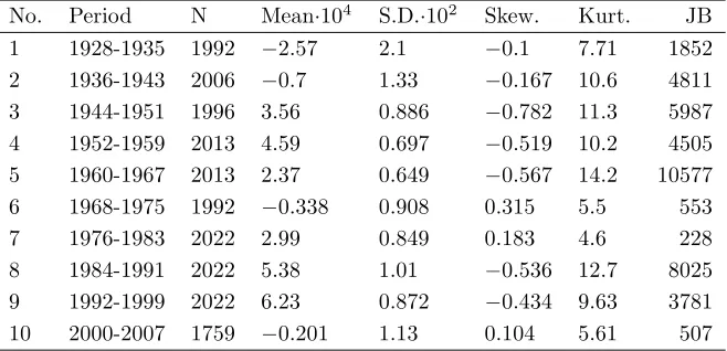
Table 1: Descriptive statistics of daily returns

This table summarizes the daily returns data of the S&P500 index, covering the period from 3 January 1928 to 13 August 2007.

No. Period N Mean·104 _S.D.·102 _{Skew. Kurt. JB}

1 1928-1935 1992 −2.57 2.1 −0.1 7.71 1852

2 1936-1943 2006 −0.7 1.33 −0.167 10.6 4811

3 1944-1951 1996 3.56 0.886 −0.782 11.3 5987

4 1952-1959 2013 4.59 0.697 −0.519 10.2 4505

5 1960-1967 2013 2.37 0.649 −0.567 14.2 10577

6 1968-1975 1992 −0.338 0.908 0.315 5.5 553

7 1976-1983 2022 2.99 0.849 0.183 4.6 228

8 1984-1991 2022 5.38 1.01 −0.536 12.7 8025

9 1992-1999 2022 6.23 0.872 −0.434 9.63 3781

10 2000-2007 1759 −0.201 1.13 0.104 5.61 507

All indices are leptokurtic. The Jarque-Bera statistic confirms the departure from normality for all return series at the 1% level of significance. In the following, we refer to the different periods by the numbers 1-10, indicated in the first column.

4

Results

The results are presented in five parts. The first part, Section 4.1 addresses model selection aspects, i.e., choice of the number of states and conditional distributions of a model. Section 4.2 summarizes some basic estimation re-sults, and in Section 4.3 we present an analysis of the stylized facts estab-lished by Granger & Ding (1995a). The content of the last part, Section 4.4, is mainly dealing with an analysis of the state-persistence of the different models.

4.1

Model selection

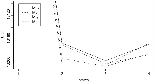
crite-ria such as AIC (Akaike Information Criterion), BIC (Bayesian Information Criterion), and modifications of both may be used (MacDonald & Zucchini 1997). Simulation studies showed that AIC tends to select models more com-plex than the true model (Visser et al. 2002), which is why we chose the BIC as main model selection tool. The following Figure 1 provides a first impres-sion as to which models are generally preferred. It shows the mean BIC over all sub-series for the four models with two to four states (lines going up on the left side result from a single Gaussian distribution). On average, MN t

with three and Mtwith two or three states show the lowest BIC values. The

BIC of MRY is permanently high, however, the values for MN are relatively

low, in particular for the models with more than 2 states.

Figure 1: BIC for 2- to 4-state-models

This figure shows the average BIC calculated from the 10 sub-series for the 4 models considered.

−13200

−13160

−13120

states

BIC

1 2 3 4

MRY

MN

MNt

Mt

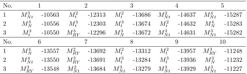
To compare the models in compact form, we denote the number of states by a superscript in what follows. Table 2 displays those three models which attain the lowest BIC together with the value of the criterion. The purely Gaussian models are selected only three times, MRY for series 7 and 10, and MN for

series 6. In the remaining cases, a model with tcomponent(s) performs best. Moreover, 20 of the 30 models displayed are not purely Gaussian, which also indicates thatMN tand Mtshould be considered for further analysis. For the

Table 2: BIC of the best fitted models

The three models with the lowest BIC, evaluated for each of the ten sub-series. The superscript indicates the number of states.

No. 1 2 3 4 5

1 M3

N t -10563 Mt2 -12313 Mt2 -13686 MN t2 -14637 MN t4 -15287

2 M3

N -10556 Mt3 -12303 Mt3 -13674 Mt2 -14632 MN4 -15283

3 M3

t -10550 MRY3 -12296 MN3 -13672 MN t3 -14631 MN t3 -15282

No. 6 7 8 9 10

1 M4

N -13557 MRY2 -13692 Mt2 -13312 Mt2 -13957 MRY3 -11248

2 M4

N t -13550 MRY3 -13691 Mt3 -13284 Mt3 -13936 MN3 -11232

3 M3

RY -13548 MN t2 -13684 MN t3 -13279 MN t3 -13929 MN t3 -11227

For the remainder of the paper, MRY serves as reference. To select the

correct number of states, we carry out two steps. At first, we chose those models which perform best according to the BIC criterion. That is, for every series we determine the preferred Mi

RY, i ∈ {2,3,4}, by the lowest criterion

value and similarly conduct the selection of one of the models Mi

N t and Mti.

Secondly, we check the stability of the estimated parameters by means of their standard error. As the Hessian does not provide numerically stable results for long time series, the standard errors are computed by a parametric bootstrap approach (Visser et al. 2000). We can partially confirm the observation of RY that the three-state models ‘are less similar to each other’ and that ‘the estimation results seem heavily dependent on outlying observations’. In our setting, the preferred 3-state models for the series 3, 8, and 9 showed a high parameter instability in the TPM (low persistence of at least one diagonal element and standard errors of up to 0.10-0.24) and thus in these cases a 2-state model is selected. For the models with t-components, the degrees of freedom often display very high standard errors. In particular, for all models with three and more states and for someM2

t, the 95%-confidence band of the

parameter ν ranged up to or close to the value 40, and thus the more stable model M2

N t is preferred. Therefore, all models selected with t-components

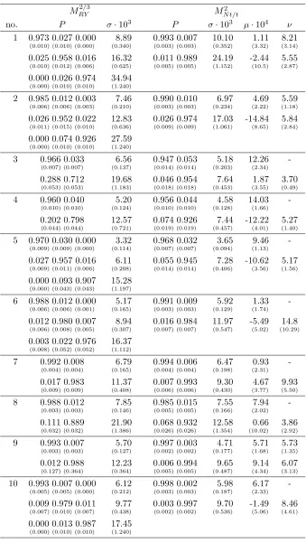
Table 3: Parameter estimates for 10 sub-series of the S&P500

Parameter estimates for the preferred models with and without t components, selected according to the BIC and parameter stability. Note that the standard deviation in the states with t-distributions requires an adjustment by the factor pν/(ν−2) for direct comparison with Gaussian states.

M_RY2/3 M2

N t/t

no. P σ·103 P σ·103 µ·104 ν

1 0.973 0.027 0.000 8.89 0.993 0.007 10.10 1.11 8.21

(0.010) (0.010) (0.000) (0.340) (0.003) (0.003) (0.352) (3.32) (3.14)

0.025 0.958 0.016 16.32 0.011 0.989 24.19 -2.44 5.55

(0.010) (0.012) (0.006) (0.625) (0.005) (0.005) (1.152) (10.5) (2.87)

0.000 0.026 0.974 34.94 (0.000) (0.010) (0.010) (1.240)

2 0.985 0.012 0.003 7.46 0.990 0.010 6.97 4.69 5.59

(0.006) (0.006) (0.003) (0.210) (0.003) (0.003) (0.234) (2.22) (1.18)

0.026 0.952 0.022 12.83 0.026 0.974 17.03 -14.84 5.84

(0.011) (0.015) (0.010) (0.636) (0.009) (0.009) (1.061) (8.65) (2.84)

0.000 0.074 0.926 27.59 (0.000) (0.010) (0.010) (1.240)

3 0.966 0.033 6.56 0.947 0.053 5.18 12.26

-(0.007) -(0.007) (0.137) (0.014) (0.014) (0.203) (2.34)

0.288 0.712 19.68 0.046 0.954 7.64 1.87 3.70

(0.053) (0.053) (1.183) (0.018) (0.018) (0.453) (3.55) (0.49)

4 0.960 0.040 5.20 0.956 0.044 4.58 14.03

-(0.010) -(0.010) (0.124) (0.010) (0.010) (0.128) (1.66)

0.202 0.798 12.57 0.074 0.926 7.44 -12.22 5.27

(0.044) (0.044) (0.721) (0.019) (0.019) (0.457) (4.01) (1.40)

5 0.970 0.030 0.000 3.32 0.968 0.032 3.65 9.46

-(0.009) -(0.009) (0.000) (0.114) (0.007) (0.007) (0.094) (1.13)

0.027 0.957 0.016 6.11 0.055 0.945 7.28 -10.62 5.17

(0.009) (0.011) (0.006) (0.208) (0.014) (0.014) (0.406) (3.56) (1.56)

0.000 0.093 0.907 15.28 (0.000) (0.043) (0.043) (1.197)

6 0.988 0.012 0.000 5.17 0.991 0.009 5.92 1.33

-(0.006) -(0.006) (0.001) (0.165) (0.003) (0.003) (0.129) (1.74)

0.012 0.980 0.007 8.94 0.016 0.984 11.97 -5.49 14.8

(0.006) (0.008) (0.005) (0.307) (0.007) (0.007) (0.547) (5.02) (10.29)

0.003 0.022 0.976 16.37 (0.008) (0.052) (0.052) (1.112)

7 0.992 0.008 6.79 0.994 0.006 6.47 0.93

-(0.004) -(0.004) (0.165) (0.004) (0.004) (0.198) (2.31)

0.017 0.983 11.37 0.007 0.993 9.30 4.67 9.93

(0.009) (0.009) (0.408) (0.006) (0.006) (0.430) (3.77) (5.50)

8 0.988 0.012 7.85 0.985 0.015 7.55 7.94

-(0.003) -(0.003) (0.146) (0.005) (0.005) (0.166) (2.02)

0.111 0.889 21.90 0.068 0.932 12.58 0.66 3.86

(0.032) (0.032) (1.386) (0.026) (0.026) (1.354) (10.02) (2.92)

9 0.993 0.007 5.70 0.997 0.003 4.71 5.71 5.73

(0.003) (0.003) (0.127) (0.002) (0.002) (0.177) (1.68) (1.35)

0.012 0.988 12.23 0.006 0.994 9.65 9.14 6.07

(0.127) (0.364) (0.364) (0.005) (0.005) (0.487) (4.34) (3.13)

10 0.993 0.007 0.000 6.12 0.998 0.002 5.98 6.17

-(0.005) -(0.005) (0.000) (0.212) (0.003) (0.003) (0.187) (2.33)

0.009 0.979 0.011 9.77 0.003 0.997 9.70 -1.49 8.46

(0.007) (0.010) (0.007) (0.438) (0.002) (0.002) (0.536) (5.06) (4.61)

Table 3 shows the parameter estimates for the selected models and the stan-dard errors of the parameters. We observe the following: First, comparing the TPM of models with and without t-component, the matrix of the latter models has more persistent states and lower standard errors with only very few exceptions (note in particular Series 4). Second, the more volatile state of Mnt/Mt has a lower conditional mean for eight of the ten series, and all

mean estimates are subject to high standard errors. We further investigate this aspect in 4.4. Third, the degrees of freedom estimates take a high value and additionally are subject to high standard deviation in Periods 6 and 7. This may indicate that in these periods an extension towards t-components may not entail in a significantly better fitted model.

Additionally to the BIC and stability checks, we apply a likelihood ratio test (LRT) to further investigate the differences between hierarchically nested models. As only the 2-state models provide stable results for most of the series, we carry out sequential tests (always at 1%-level) for these models, starting with M2

RY and MN2. For this comparison, MN turns out to be the

a significantly better model for six of the ten periods. Proceeding with the comparison of M2

N and MN t2 , the latter is preferred in nine periods. As the

parameter estimates already indicated, the simpler model is preferred in Pe-riod 6. The last test between M2

N t and Mt2 shows that the more complex

model is selected in five cases.

Summarizing this section, the extension from the common HMM utilizing Gaussian components with identical means to models with varying means and at least one conditional t-distribution seems to be reasonable. Often these models are more parsimonious than a Gaussian 3-state alternative, provide more stable parameter estimates, and are preferred by both the BIC and the LRT.

4.2

Basic statistics

To continue the analysis, we present some basic statistics on the returns and model selection criteria. For most series, the degrees of freedom ν of the

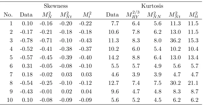
t-distributions take low values, indicating a departure from normality in the components. As to the fit of the models to the empirical distribution of the returns, Table 4 summarizes empirical and model skewness, and kurtosis. All models experience minor problems in reproducing a positive skewness, while negatively skewed series are mostly reproduced well. Moreover, it should be noted that MRY is, by construction of the model, not able to reproduce any

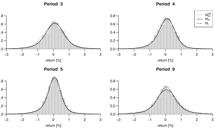
Figure 2: Empirical distribution and model densities for selected periods

Empirical distributions with model densities, Periods 3, 4, 5, and 9. In Period 5,MRY is a

3-state model. We do not displayMN, because there is only a very small visual difference

to MRY.

return [%]

−3 −2 −1 0 1 2 3

0.0 0.2 0.4 0.6 0.8

Period 3

return [%]

−3 −2 −1 0 1 2 3

0.0 0.2 0.4 0.6 0.8

Period 4

MRY 2 3

MNt

Mt

return [%]

−3 −2 −1 0 1 2 3

0.0 0.2 0.4 0.6 0.8

Period 5

return [%]

−3 −2 −1 0 1 2 3

0.0 0.2 0.4 0.6 0.8

Period 9

the mean of the fitted models both lie very close to zero for all series, and the standard deviation almost coincides with the empirical value for each model. Table 4 displays skewness and kurtosis for the models considered. Application of Friedman’s rank sum test to test for the equality of mean, standard deviation, skewness and kurtosis location of data and models rejects the hypothesis for skewness and kurtosis. However, further investigation of the skewness of the sample data and each model by paired two sample Wilcoxon tests does not reveal any significant differences. As to the kurtosis, the Wilcoxon test rejects the equality hypothesis for the data andMRY as well

as MN at 1% and 5% level, respectively. This confirms the first impression

from the Figure 2 that the Gaussian models do not seem to reproduce the kurtosis.

Additionally, regarding Series 1, 2, 5, 6, and 10, the Gaussian models with three states do not seem to reproduce the Kurtosis better than M2

RY/MN2

Table 4: Skewness and kurtosis for the data and fitted models

Skewness and kurtosis of the returns and the four fitted modelsMRY (skewness omitted,

equals zero),MN N,MN t, andMtt(by Monte Carlo approximation).

Skewness Kurtosis

No. Data M2

N MN t2 Mt2 Data M 2/3

RY MN N2 MN t2 Mtt2

1 0.10 -0.16 -0.20 -0.22 7.7 6.4 5.6 11.3 11.5

2 -0.17 -0.21 -0.18 -0.18 10.6 7.8 6.2 13.0 11.5

3 -0.78 -0.71 -0.10 -0.43 11.3 8.3 8.0 36.2 15.3

4 -0.52 -0.41 -0.38 -0.37 10.2 6.0 5.4 10.2 10.4

5 -0.57 -0.45 -0.39 -0.40 14.2 8.8 6.4 13.0 13.4

6 0.31 -0.05 -0.08 -0.10 5.5 5.7 4.9 5.6 5.7

7 0.18 -0.02 0.03 0.03 4.6 3.9 3.9 4.7 4.7

8 -0.54 -0.25 -0.10 -0.12 12.7 7.4 7.5 30.2 21.1

9 -0.43 -0.01 0.02 0.04 9.6 4.7 4.8 8.3 8.7

10 0.10 -0.08 -0.09 -0.09 5.6 5.2 4.5 6.2 6.2

The paper of Breunig et al. (2003) presents tests on mean, variance and peak location. The basic idea of these encompassing tests is to check the hypothesis that a parameter ˆγ that has been estimated from the data is reproduced by the model. The null hypothesis is that the model is correct, and the test statistic is

R= (ˆγ−γM(ˆθ))t[var(ˆγ)]−1(ˆγ−γM(ˆθ)),

following a χ2

dim(ˆγ) distribution. The quantity ˆθ is the MLE estimate of

the model parameters, and γM(ˆθ) the model quantity corresponding to ˆγ.

According to the proposals of Breunig et al. (2003), γM(ˆθ) and var(ˆγ) are

estimated by simulation techniques. An analysis of mean and variance does not reveal any differences between the models, all perform comparably well. However, the authors also propose a test statistic

ˆ

φ=T−1 T

X

t=1

1(−k,k)(xt),

of 4%, because some of the series do not contain any observations for bigger integer values.

Table 5: Measures for outlier fraction in data and models

Results for quantity ˆφ∗

= T−1PT

t=11[4,∞)(|xt|) (in %) and corresponding values of R.

The critical value forR at 5% and 1% level is 3.84 and 6.63, respectively.

Data M_RY2/3 R M2

N R MN t2 R Mt2 R

1 6.07 6.66 5.43 7.03 13.91 6.02 0.06 6.15 0.11

2 1.69 1.80 0.61 1.80 0.57 1.67 0.05 1.71 0.01

3 0.40 0.43 0.24 0.39 0.02 0.42 0.10 0.46 0.89

4 0.10 0.02 23.46 0.01 126.55 0.10 0.00 0.10 0.00

5 0.10 0.07 0.99 0.01 131.48 0.09 0.07 0.10 0.00

6 0.20 0.19 0.08 0.08 20.44 0.16 1.11 0.16 0.97

7 0.10 0.01 53.82 0.02 41.89 0.07 1.01 0.07 1.07

8 0.54 0.67 2.42 0.66 2.19 0.62 0.92 0.59 0.33

9 0.25 0.04 117.10 0.04 104.97 0.23 0.20 0.23 0.15

10 0.57 0.61 0.26 0.39 7.79 0.66 1.39 0.67 1.43

The modelsMRY andMN are rejected 4 and 7 times, respectively, at 5% level.

The models with t-distributions are not rejected at all, indicating that they are more capable to reproduce daily return series with extreme observations.

Summarizing, MN tand Mtallow for skewed distributions, and reproduce the

kurtosis as well as extreme observations better than their competitors with Gaussian components. In this connection, note that three-state Gaussian models are also affected by the weaker performance.

4.3

Stylized facts

In their article on stylized facts of daily return series and the HMM, Ryd´en et al. (1998) analyze their model’s ability to reproduce four temporal and three distributional properties of daily returns. Their main result is that

MRY reproduces most of the properties quite well, with exception of the very

slow decay of the autocorrelation function of absolute or squared returns. In this section, we check these properties for MN, MN t, and Mt. The

TP1: Returns rt are not autocorrelated (except for, possibly, at

lag one)

TP2: |rt| and rt2 are ’long-memory’, i.e., their autocorrelation

functions decay slowly starting from the first autocorrela-tion, and corr(|rt|,|rt−k|) > corr(rt2, r2t−k). The

autocor-relations remain positive for many lags and the decay is much slower than the exponential rate of a typical station-ary ARMA model.

TP3: The Taylor effect corr(|rt|,|rt−k|)>corr(|rt|θ,|rt−k|θ), θ 6=

1 (Taylor 1986). Autocorrelations of powers of absolute returns are highest at power one.

TP4: The autocorrelations of sign(rt) are negligibly small.

The three distributional properties are: DP1: |rt| and sign(rt) are independent.

DP2: Mean |rt| = standard deviation |rt|.

DP3: The marginal distribution of |rt| is exponential (after outlier

correc-tion).

Note that an exponentially distributed variable (DP3) xt has the following

properties.

PED1: E(xt) =V ar(xt) (same as DP2).

PED2: E(xt−E(xt))3 = 2.

PED3: E(xt−E(xt))4 = 9.

In their analysis, RY showed that MRY satisfies TP1, and that TP4 is not

violated in practice. Moreover, DP1 holds by construction of the model. Al-thoughMN,MN t, andMthave means unequal to zero, all conditional means

take values very close to zero. As expected, a preliminary analysis showed that none of the estimated models violates TP1, TP4 or DP1.

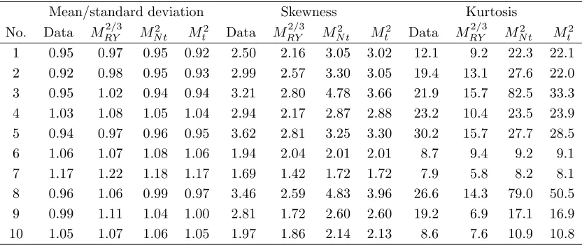
We firstly analyze PED1-PED3: Table 6 presents the mean-standard devi-ation ratio, skewness, and kurtosis of the absolute returns and the fitted models (we omitMN, as the results are almost similar toMRY). The ratio of

mean and standard deviation (PED1/DP2) is close to one for all series and all fitted models, however, sometimes slightly overestimated by the models with two Gaussian components. This is in line with the analysis of RY, who noted that PED1 ‘has to be relaxed somewhat (the mean has to be allowed to be slightly larger than the standard deviation) if we at the same time want PED2 and PED3 to be satisfied’. For the original data,MRY andMN

these stylized facts quite well with a slightly better performance of the latter one. Skewness and kurtosis are reproduced considerably well by all models. For some series, MRY and MN slightly underestimate these moments, while

MN t and Mt sometimes overestimate them.

To summarize the above findings, MN t and Mt reproduce PED1-PED3 as

well as or better than MRY and MN for the original data.

Table 6: Statistics of the absolute returns and the estimated models

Mean-standard deviation ratio, skewness and kurtosis of the absolute returns estimated from the ten data series and from the fitted modelsMRY,MN t, andMt(by Monte Carlo approximation)

Mean/standard deviation Skewness Kurtosis

No. Data M_RY2/3 M2

N t Mt2 Data M 2/3

RY MN t2 Mt2 Data M 2/3

RY MN t2 Mt2

1 0.95 0.97 0.95 0.92 2.50 2.16 3.05 3.02 12.1 9.2 22.3 22.1

2 0.92 0.98 0.95 0.93 2.99 2.57 3.30 3.05 19.4 13.1 27.6 22.0

3 0.95 1.02 0.94 0.94 3.21 2.80 4.78 3.66 21.9 15.7 82.5 33.3

4 1.03 1.08 1.05 1.04 2.94 2.17 2.87 2.88 23.2 10.4 23.5 23.9

5 0.94 0.97 0.96 0.95 3.62 2.81 3.25 3.30 30.2 15.7 27.7 28.5

6 1.06 1.07 1.08 1.06 1.94 2.04 2.01 2.01 8.7 9.4 9.2 9.1

7 1.17 1.22 1.18 1.17 1.69 1.42 1.72 1.72 7.9 5.8 8.2 8.1

8 0.96 1.06 0.99 0.97 3.46 2.59 4.83 3.96 26.6 14.3 79.0 50.5

9 0.99 1.11 1.04 1.00 2.81 1.72 2.60 2.60 19.2 6.9 17.1 16.9

10 1.05 1.07 1.06 1.05 1.97 1.86 2.14 2.13 8.6 7.6 10.9 10.8

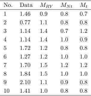
The two remaining stylized facts are TP3 and TP2. For TP3, the Tay-lor effect, we estimate the coefficient θ for every period by maximizing the first-order autocorrelation of |rt|θ utilizing numerical optimization routines.

Following the approach of RY, the value ofθmaximizing the first-order auto-correlation for the models was estimated over the range{0.1, 0.2, . . . , 2.0}by Monte-Carlo approximation. Table 7 summarizes the results, and again the results forMN are not displayed as they are similar to those ofMRY. On the

Table 7: Taylor coefficient of the returns and the estimated models

Values ofθmaximizing the first-order autocorrelation of|rt|θestimated from the ten return

series and the fitted models.

No. Data MRY MN t Mt

1 1.46 0.9 0.8 0.7

2 0.77 1.1 0.8 0.8

3 1.14 1.4 0.7 1.2

4 1.14 1.4 1.0 0.9

5 1.72 1.2 0.8 0.8

6 1.27 1.2 1.0 1.0

7 1.70 1.5 1.2 1.2

8 1.84 1.5 1.0 1.0

9 2.10 1.1 0.9 0.8

10 1.41 1.0 0.8 0.8

According to RY, the slow decay of the ACF for series of absolute daily returns, which is stylized fact TP2, cannot be reproduced by the HMM be-cause the decay of the autocorrelations is (much) faster than that observed in reality. They considered this stylized fact to be ‘the most difficult [...] to reproduce with a HMM’. Figures 3 and 4 show the empirical ACF and the ACF of the the fitted models (we do not display MN, because it is visually

indistinguishable from MRY). The left and right panels display models with

2 and 3 states, respectively. The solid line represents the ACF of MRY, the

dashed corresponds to MN t and the dotted lines to Mt.

In most cases, the ACF of MRY shows a much stronger decay of the

autocor-relations than the decay of the empirical ACF, which confirms the results of RY. The models witht-components reproduce this stylized fact much better, although their fit show slight deficiencies for lower lags in most of the peri-ods. However, it also seems that models with three states provide a better fit than models with two states. To verify these visual impressions, we measure the fit of the ACF by the mean squared error (MSE). Table 8 displays the results. The average MSE over all periods is denoted by MSE; MSEl and

MSEh represent the MSE for the ’lower’ lags 1-20 and ’higher’ lags 21-100,

respectively. The MSE confirm the visual impression that models with three and at least one conditional t-distribution provide the best fit, especially for the lags of higher order. If a model with two states is preferred, Mt would

Figure 3: Empirical and model ACF of absolute returns for Series 1-5, lag 1-100

The panels show the empirical ACF of absolute returns (grey bars) and the model ACF (straight line for MRY, dashed line for MN t, and dotted line for Mt). Models with two

and three states are displayed in the left and right panels, respectively. We omit MN,

because there is almost no visual difference toMRY.

20 40 60 80 100

0.00

0.10

0.20

lag

ACF

Period 1

MRY 2 MNt 2 Mt 2

20 40 60 80 100

0.00 0.10 0.20 lag ACF MRY 3 MNt 3 Mt 3

20 40 60 80 100

0.00

0.10

0.20

lag

ACF

Period 2

20 40 60 80 100

0.00

0.10

0.20

lag

ACF

20 40 60 80 100

0.00

0.10

0.20

lag

ACF

Period 3

20 40 60 80 100

0.00

0.10

0.20

lag

ACF

20 40 60 80 100

0.00

0.10

0.20

lag

ACF

Period 4

20 40 60 80 100

0.00

0.10

0.20

lag

ACF

20 40 60 80 100

0.00

0.10

0.20

lag

ACF

Period 5

20 40 60 80 100

0.00

0.10

0.20

lag

Figure 4: Empirical and model ACF of absolute returns for Series 6-10, lag 1-100

The panels show the empirical ACF of absolute returns (grey bars) and the model ACF (straight line for MRY, dashed line for MN t, and dotted line for Mt). Models with two

and three states are displayed in the left and right panels, respectively. We omit MN,

because there is almost no visual difference toMRY.

20 40 60 80 100

0.00

0.10

0.20

lag

ACF

Period 6

MRY 2 MNt 2 Mt 2

20 40 60 80 100

0.00 0.10 0.20 lag ACF MRY 3 MNt 3 Mt 3

20 40 60 80 100

0.00

0.10

0.20

lag

ACF

Period 7

20 40 60 80 100

0.00

0.10

0.20

lag

ACF

20 40 60 80 100

0.00

0.10

0.20

lag

ACF

Period 8

20 40 60 80 100

0.00

0.10

0.20

lag

ACF

20 40 60 80 100

0.00

0.10

0.20

lag

ACF

Period 9

20 40 60 80 100

0.00

0.10

0.20

lag

ACF

20 40 60 80 100

0.00

0.10

0.20

lag

ACF

Period 10

20 40 60 80 100

0.00

0.10

0.20

lag

Table 8: Average mean squared error of the ACF for absolute returns

Mean squared error of the empirical and the model ACF, averaged over the ten periods of the S&P500. The error for the lags 1-100 is denoted by M SE, whileM SEl andM SEh

represent the mean squared error for the lags 1-20 and 21-100, respectively. All errors are scaled by 104_.

2 states 3 states

Criterion M SE M SEl M SEh M SE M SEl M SEh

MRY 3.48 2.93 3.62 2.3 1.34 2.54

MN t 3.96 5.21 3.64 2.19 1.95 2.25

Mt 2.97 4.03 2.70 1.95 1.80 1.99

Summarizing,MN tandMtreproduce most of the temporal and distributional

properties as well as or better than MRY and MN. In particular, the models

with conditional t-distributions are able to reproduce the slow decay of the ACF of absolute returns much better than the models with two Gaussian distributions.

A final remark on the impact of outliers: According to Chan (1995) extreme outliers could jeopardize the specification power of the ACF. To analyze outlier effects, we followed the approach of Granger & Ding (1995a) and gen-erated a second data set by setting values outside the interval [¯rt−4ˆσ,r¯t+4ˆσ]

equal to the value of the closest interval boundary. Here, ˆσ and ¯rtdenote the

estimated standard deviation and mean, respectively. However, the results from this second data set have not produced much additional insight: Con-cerning the ACF, the outlier-corrected data show similar results. As to the Taylor effect, we can confirm the observation of RY that outlier-correction weakens the Taylor effect (the median ofθincreases from 1.43 to 1.57). With respect to the statistics on distributional properties of absolute returns, the outlier-correction causes a reduction of the differences between the models.

4.4

Persistence of stock market volatility

itself can also be used to predict changes in the economic variables, such as GDP growth (Campbell et al. 2001). In the following, we investigate the ability of our models to reproduce these two findings by means of the ten sub-series of the S&P 500, and an additional analysis of the S&P500, the German DAX30, French CAC40, Swiss SMI, and Japanese Nikkei225 for a 15-year period from 1993 to 2007.

Similar to Section 4.1, the models are selected by the BIC and parameter stability in terms of low standard error. To keep the results from differ-ent models comparable for each index, we fit models with two states to the S&P500, SMI, and Nikkei, and 3-state models to DAX and CAC. Table 12 and 13 in the Appendix show the parameter estimates and BIC values, re-spectively (we omit the results forMN as they are very close to MRY). Note

that in case of the DAX, the third state of MRY is rather non-persistent

- however, for the models with t-component all three states are persistent. According to the BIC criterion, either Mt or MN t or both are preferred for

the S&P500, DAX, CAC, whereas for SMI and Nikkei the Gaussian models seem sufficient.

The ability of MN,MN t, andMt to link periods of high volatility to periods

of falling stock prices can be deduced directly from the estimated parame-ters. As shown in Tables 3 and 12, the conditional mean of the state with low/medium standard deviation is higher than the conditional mean of the state with high standard deviation (in the following, we refer to these states by ’low-risk state’, ’medium-risk state’ and ’high-risk state’). Moreover, the conditional mean of the high-risk state is negative and the mean for the low/medium-risk state positive for the large majority of indices and periods considered. An exception seems to be Periods 7 and 9, where the models incur difficulties to establish the link between high volatility and low return. As the conditional means ofMRY are both zero, it is not possible to establish

a direct relation between high volatility and low returns for this model. In what follows, we focus on the so-called ’smoothing probabilities’, which are given by

P(St=i|X₁T)

fori∈ {1, ..., m}andt∈ {1,· · · , T}. These probabilities are a by-product of the EM algorithm, for their derivation we refer to Appendix B and the refer-ences mentioned therein. The evolution of the hidden state sequence is often a key analysis tool, as the states are linked to an economic interpretation (see, e.g. Guidolin & Timmermann 2005, Linne 2002, Maheu & McCurdy 2001). The following Tables 9 and 10 illustrate the effect of including conditional

visit. The state visited is determined by arg max

j P(St=j|X T

1). Again,MN

is omitted as the difference toMRY is very low. The states are denoted by ’lr’

and ’hr’ for high- and low-risk, for 3-state models additionally ’mr’ (medium-risk) exists. A notable effect is that the persistence of all states increases when

Mt is used instead ofMRY. ForMN t, the results differ slightly: Compared to

MRY, the persistence of the high-risk state consistently increases. However,

this is not always the case for the low-/medium-risk states. Note that for some sub-series the effects are even stronger.

Table 9: Average estimated sojourn times, 2-state models

Estimated sojourn times per state in trading days for the ten periods (averaged) and S&P500, SMI, and Nikkei for the period 1993-2007. The states denoted ’lr’ (low risk) and ’hr’ (high risk) correspond lower respectively higher conditional standard deviations.

sub-series S&P500 SMI Nikkei

Model lr hr lr hr lr hr lr hr

MRY 111 54 115 72 218 36 128 59

MN t 132 102 126 126 138 49 127 83

Mt 201 111 350 280 254 66 148 92

Table 10: Average estimated sojourn times, 3-state models

Estimated sojourn times per state in trading days for DAX and CAC for the period 1993-2007. The states denoted ’lr’ (low risk), ’mr’ (medium risk), and ’hr’ (high risk) correspond lower, medium, and higher conditional standard deviations, respectively.

DAX CAC

Model lr mr hr lr mr hr

MRY 230 27 5 94 60 24

MN t 171 21 25 91 59 54

Mt 305 46 14 174 81 58

they allow for a higher robustness towards short periods of observations with comparably high volatility.

Figure 5 visualized the effect of adding conditional t-distributions by plot-ting the smoothing probabilities and resulplot-ting state classifications. The top eight panels display the returns and smoothing probabilities for the S&P500 on the left and for the Nikkei on the right. For better identification, the background of the periods with P(St= 2)> P(St= 1) is shaded light gray.

These two 2-state models visualize how large respectively small the effect of conditional t-distributions can be. The state classification of the S&P500 changes completely as the number of transitions (or state switches) reduces from 41 (MRY) to 23 (MN t) and finally 5 (Mt). In case of the Nikkei, however,

the (optical) difference between the models is much smaller. The lower eight panels show corresponding quantities resulting from the two 3-state mod-els for CAC and DAX. The solid and dotted lines represent P(St = 2) and

P(St = 3) respectively, and the background of the high-risk state is shaded

dark grey. For both indices, the evolution of the estimated state sequence changes considerably.

Recapitulating, the parameter estimates for MN, MN t, and Mt confirm the

link between periods of high volatility and falling stock prices. Moreover, the persistence of most regimes increases significantly when substituting the com-monly used Gaussian conditional distributions by at least one t-distributed component. This gives rise to longer estimated periods with high, respec-tively low and medium stock volatility. Finally, the state evolution of the models with conditionalt-distribution, which are often preferred by the BIC, changes considerably compared to MRY.

5

Conclusion

In this paper we present an amelioration of the common HMM with condi-tional Gaussian distributions by introducing condicondi-tionalt-distributions. This includes models with varying distributions in different states, which have not been analyzed yet in the context of daily return series.

By means of an application to the S&P 500 index, we show that, in par-ticular, HMMs with varying conditional mean and at least one conditional

proba-Figure 5: International indices with smoothing probabilities, 1993-2007

The figure shows percentage returns of the S&P 500, Nikkei, CAC, and DAX from 1993 to 2007. Below each return series, three panels display the corresponding the smoothing probabilities P(St = i|X1T) for MRY, MN t, and Mt, respectively. The background of

periods with ˆst= 2 is shaded light gray. For the two 3-state models (DAX and CAC), the

background of periods with ˆst= 3 is shaded dark gray. The smoothing lines themselves

are solid and dotted for state 2 and 3, respectively. We omitMN, because there is almost

no visual difference toMRY.

trading day

return (%)

−4 0 4

1000 2000 3000 S&P 500

93 94 95 96 97 98 99 00 01 02 03 04 05 06 07

1000 2000 3000

0.0

0.4

0.8

trading day

sm. prob.

MRY trans: 41

1000 2000 3000

0.0

0.4

0.8

trading day

sm. prob.

MNt trans: 23

1000 2000 3000

0.0

0.4

0.8

trading day

sm. prob.

Mt trans: 5

trading day

return (%)

−4

0

4

1000 2000 3000 Nikkei

93 94 95 96 97 98 99 00 01 02 03 04 05 06 07

1000 2000 3000

0.0

0.4

0.8

trading day

sm. prob.

MRY trans: 38

1000 2000 3000

0.0

0.4

0.8

trading day

sm. prob.

MNt trans: 39

1000 2000 3000

0.0

0.4

0.8

trading day

sm. prob.

Mt trans: 33

trading day

return (%)

−4

0

4

1000 2000 3000 CAC

93 94 95 96 97 98 99 00 01 02 03 04 05 06 07

1000 2000 3000

0.0

0.4

0.8

trading day

sm. prob.

MRY trans: 57

1000 2000 3000

0.0

0.4

0.8

trading day

sm. prob.

MNt trans: 51

1000 2000 3000

0.0

0.4

0.8

sm. prob.

Mt trans: 39

trading day

return (%)

−4

0

4

1000 2000 3000 DAX

93 94 95 96 97 98 99 00 01 02 03 04 05 06 07

1000 2000 3000

0.0

0.4

0.8

trading day

sm. prob.

MRY trans: 38

1000 2000 3000

0.0

0.4

0.8

trading day

sm. prob.

MNt trans: 43

1000 2000 3000

0.0

0.4

0.8

sm. prob.

bility mass around zero and heavy tails of the t-distribution. It allows for a higher robustness towards short periods lower or higher volatility when the actual regime actually is a high- respectively low-volatile regime residing in a (very) short period of contrary pattern.

An analysis of various international indices equally shows that the inclu-sion of conditional t-distributions often lowers the BIC significantly. More importantly, the evolution of the estimated state sequence by smoothing probabilities changes considerably. As the estimated state sequence is often utilized to link certain economic patterns to particular periods, conditional

APPENDIX

Table 13: BIC values for return series 1993-2007, 3-state models

BIC values for the four modelsMRY,MN,MN t, andMt. For DAX and CAC results are

from 3-state models, for the other series from 2-state models.

Model S&P500 DAX CAC SMI Nikkei

Table 11: BIC values for S%P500 sub-series, 2- to 4-state models

BIC values for the four modelsMRY,MN,MN t, andMt. The upper part of the table displays 2-state-models, the

middle and lower part show 3- and 4-state-models, respectively.

States Model 1 2 3 4 5 6 7 8 9 10

MRY -10473 -12265 -13630 -14563 -15175 -13517 -13692 -13255 -13874 -11218

MN -10464 -12257 -13652 -14599 -15203 -13503 -13680 -13256 -13877 -11206

2

MN t -10489 -12286 -13662 -14637 -15253 -13500 -13684 -13273 -13924 -11214

Mt -10501 -12313 -13686 -14632 -15251 -13497 -13676 -13312 -13957 -11208

MRY -10535 -12296 -13656 -14558 -15248 -13548 -13691 -13263 -13920 -11248

MN -10556 -12283 -13672 -14612 -15279 -13529 -13673 -13257 -13915 -11232

3

MN t -10563 -12284 -13667 -14631 -15282 -13521 -13669 -13279 -13929 -11227

Mt -10550 -12303 -13674 -14619 -15267 -13534 -13653 -13284 -13936 -11211

MRY -10528 -12262 -13634 -14515 -15225 -13513 -13643 -13235 -13917 -11214

MN -10545 -12243 -13661 -14605 -15283 -13557 -13629 -13249 -13899 -11191

4

MN t -10536 -12248 -13665 -14611 -15287 -13550 -13624 -13242 -13898 -11183

Mt -10515 -12251 -13636 -14594 -15268 -13525 -13600 -13229 -13890 -11160

Table 12: Parameter estimates for international indices, 1993-2007

Parameter estimates for the preferred modelsMRY, Mnt, andMt. Note that the standard deviation in the states with t-distributions

requires an adjustment by the factor pν/(ν−2) for direct comparison with Gaussian states.

M_RY2/3 M_{N t}2/3 Mt2/3

Index P σ·103 P σ·103 µ·104 ν P σ·103 µ·104 ν

S&P500 0.990 0.010 6.36 0.992 0.008 5.93 7.19 0.998 0.002 5.34 6.90 6.52

(0.004) (0.004) (0.14) (0.004) (0.004) (0.15) (2.05) (0.002) (0.002) (0.22) (1.99) (2.51)

0.016 0.984 13.74 0.009 0.991 10.15 0.49 5.5 0.003 0.997 10.24 1.45 5.38

(0.006) (0.006) (0.42) (0.004) (0.004) (0.45) (4.19) (1.56) (0.004) (0.004) (0.49) (4.31) (1.66)

DAX 0.978 0.021 0.001 9.49 0.972 0.013 0.014 9.12 13.52 0.985 0.014 0.001 8.71 14.50 11.67

(0.007) (0.007) (0.003) (0.28) (0.012) (0.013) (0.007) (0.33) (3.63) (0.006) (0.006) (0.003) (0.37) (3.34) ( 8.91)

0.031 0.953 0.016 18.14 0.059 0.933 0.008 15.83 26.25 0.018 0.976 0.006 15.55 2.49 8.32

(0.005) (0.008) (0.006) (0.77) (0.038) (0.047) (0.026) (1.32) (14.45) (0.009) (0.026) (0.022) (1.01) (8.87) (8.55)

0.000 0.178 0.822 41.13 0.000 0.039 0.961 18.42 -32.84 4.48 0.000 0.044 0.956 24.73 -53.46 4.33

(0.000) (0.103) (0.103) (5.40) (0.001) (0.047) (0.047) (1.73) (18.05) (2.83) (0.005) (0.086) (0.085) (5.86) (75.44) (12.49)

CAC 0.991 0.009 0.000 5.60 0.989 0.011 0.000 5.44 7.08 0.994 0.006 0.000 4.62 6.69 5.51

(0.004) (0.004) (0.000) (0.15) (0.006) (0.006) (0.001) (0.17) (2.13) (0.005) (0.005) (0.000) (0.23) (2.12) (2.09)

0.010 0.980 0.010 10.48 0.013 0.978 0.009 9.79 3.42 0.007 0.983 0.009 9.33 4.78 23.43

(0.005) (0.008) (0.006) (0.36) (0.006) (0.010) (0.006) (0.37) (3.87) (0.005) (0.028) (0.027) (0.43) (4.73) (12.03)

0.000 0.046 0.954 20.08 0.000 0.021 0.979 14.90 -9.32 8.14 0.000 0.021 0.979 14.98 -10.18 8.31

(0.000) (0.059) (0.059) (1.97) (0.002) (0.021) (0.021) (1.37) (11.63) (9.93) (0.000) (0.064) (0.064) (1.55) (20.46) (11.38)

SMI 0.994 0.006 8.35 0.989 0.011 7.10 10.00 0.992 0.008 6.94 9.8 10.21

(0.002) (0.002) (0.17) (0.004) (0.004) (0.16) (2.23) (0.003) (0.003) (0.23) (2.03) (5.17)

0.021 0.979 22.7 0.018 0.982 15.23 -5.93 5.68 0.018 0.982 17.05 -9.0 6.70

(0.009) (0.009) (0.78) (0.006) (0.006) (0.75) (6.36) (1.71) (0.007) (0.007) (0.90) (8.38) (4.37)

Nikkei 0.992 0.008 6.69 0.992 0.008 6.37 6.13 0.992 0.008 6.24 6.16 40.0

(0.003) (0.003) (0.14) (0.003) (0.003) (0.14) (1.89) (0.003) (0.003) (0.16) (1.95) (9.46)

0.018 0.982 15.26 0.013 0.987 12.61 -3.75 8.61 0.013 0.987 12.69 -3.72 8.7

(0.007) (0.007) (0.50) (0.006) (0.006) (0.62) (5.15) (4.79) (0.006) (0.006) (0.62) (5.64) (5.76)

B

Re-estimation formulae

The EM algorithm has been treated in detail by many authors and we there-fore omit explicit derivations of the Q-function and re-estimation formulae. For a short overview, the article of Ephraim & Merhav (2002) and the sources mentioned therein provide a good introduction. A more comprehensive and detailed survey on HMMs was written by Capp´e et al. (2007).

The Q-function of a HMM is given by

Q(θ, θ(k)_{) =} m

X

i=1

log πiγi(1)

| {z }

A

+

m

X

i,j=1 T−1

X

t=1

log pijξij(t)

| {z }

B + m X i=1 T X t=1

γi(t) logbi(xt)

| {z }

C

,

where

γi(t) := P(St=i|X1T =xT1),

ξij(t) := P St =i, St+1 =j|X1T =x T 1

, bi(xt) := P(Xt=xt|St=i)

for i= 1, . . . , mand t = 1, . . . , T.

Transition and initial probabilities

Most implementations of the EM algorithm in the context of HMMs base on the algorithms of Baum et al. (1970). These allow to fit a homogeneous, but non-stationary HMM. For the non-stationary case, the Q-function is split up into the three additive parts denoted by A (initial component), B (tran-sition component) and C (observation component), which are maximized separately.

In order to fit a stationary Markov chain, component A and B have to be treated simultaneously, respecting a stationarity constraint. Then, the joint M-step for these two components becomes

max

pij∈Π

m

X

i=1

log πiγi(1) + m

X

i,j=1 T−1

X

t=1

log pijξij(t)

!

with πΠ˜ = (0, . . . ,0,1).

system of equations is more difficult to solve than it appears at first glance. However, solving it with numerical methods is straightforward. Compared to the original algorithms of Baum et al. (1970), the estimation does not slow down significantly. For further details on this part we refer to Bulla & Berzel (2008).

Conditional Gaussian distribution

The re-estimation formulae for the conditonal mean µi and variance σ2i of

normal component distributions are

µ(_ik+1) =

PT

t=1γi(t)xt

PT

t=1γi(t)

,

σ2i (k+1)

=

PT

t=1γi(t)

xt−µ (k+1) j

2

PT

t=1γi(t)

.

Conditional t-distribution

The maximization of the Q-function for t-distributed variables is slightly more difficult than the Gaussian case. Peel & McLachlan (2000) present some techniques for the estimation of mixtures of t-distributions, which can be adopted to HMMs with a reasonable amount of effort. For details to this step, see Bulla & Bulla (2006), where the approach is discussed for hidden semi-Markov models.

Let the density of the t-distribution with meanµ, ν degrees of freedom and positive definite inner product matrix Σ be given by

f(xt) =

Γ(ν+₂p)|Σ|−1₂ (πν)12pΓ(ν

2){1 +δ(xt,µ,Σ)/ν} 1 2(ν+p)

,

where δ(x,µ,Σ) denotes the Mahalanobis distance, defined by

δ(x,µ,Σ) = (x−µ)Σ−1_(x−µ),

and p the dimension of the observations. The re-estimation formulae forµ_i

and Σi can be derived explicitly as

µ(_ik+1) =

PT

t=1γi(t)u (k) i (t)xt

PT

and

Σ(_ik+1) =

PT

t=1γi(t)u( k)

i (t)(xt−µ( k+1)

i )(xt−µ( k+1)

i )T

PT

t=1γi(t)

,

where u(_ik)(t) denotes an auxiliary variable defined

u(_ik)(t) := νj

(k)_+p

νj(k)+δ(x (k)

t ,µ(k),Σ(k))

.

The denominator in the re-estimation equation for Σ(_ik+1) may also be re-placed by PT_t=1γi(t)u(

k)

i (t) to increase the speed of convergence (Kent et al.

1994).

The re-estimation of ν_i(k+1) is not possible explicitly. It requires determining the (unique) solution of the equation

−ψ

1 2ν

(k) i + log 1 2ν

(k) i

+ 1

+_PT 1

t=1γi(t)

" _T X

t=1

γi(t)

logu(_ik)(t)−u(_ik)(t)

#

+ψ ν

(k)

i +p

2

!

−log ν

(k)

i +p

2

!

= 0.

The solution can be determined without relevant complications, e.g., by a bisection algorithm or quasi-Newton methods, because the function on the left hand side is monotonically increasing in ν_i(k).

Conditional Gaussian and t-distributions in different states

The extension to state-varying conditional distributions is straightforward. The forward-backward pass through the observations has to be carried out re-specting the different conditional distributions. The calculation of the quan-tities γi(t), ξij(t), and bi(t) follows directly from this step. The M-step is

References

Baum, L. E. & Petrie, T. (1966), ‘Statistical inference for probabilistic func-tions of finite state Markov chains’, Ann. Math. Statist. 37, 1554–1563. Baum, L. E., Petrie, T., Soules, G. & Weiss, N. (1970), ‘A maximization

technique occurring in the statistical analysis of probabilistic functions of Markov chains’, Ann. Math. Statist. 41, 164–171.

Bialkowski, J. (2003), ‘Modelling returns on stock indices for western and central european stock exchanges - Markov switching approach’,Southeast.

Eur. J. Econ.2(2), 81–100.

Breunig, R., Najarian, S. & Pagan, A. (2003), ‘Specification testing of markov switching models’, Oxford Bull. Econ. Statist. 65(Supplement), 703–725. Bulla, J. & Berzel, A. (2008), ‘Computational issues in parameter estimation

for stationary hidden Markov models’, Computation. Stat. 23(1), 1–18. Bulla, J. & Bulla, I. (2006), ‘Stylized facts of financial time series and hidden

semi-Markov models’, Comput. Statist. Data Anal.51(4), 2192–2209. Campbell, J. Y., Lettau, M., Malkiel, B. G. & Xu, Y. (2001), ‘Have individual

stocks become more volatile? an empirical exploration of idiosyncratic risk’, J. Financ. 56(1), 1–43.

Capp´e, O., Moulines, E. & Ryden, T. (2007), Inference in Hidden Markov

Models, Springer Series in Statistics, Springer-Verlag, New York -

Heidel-berg - Berlin.

Cecchetti, S. G., Lam, P.-S. & Mark, N. C. (1990), ‘Mean reversion in equi-librium asset prices’, Am. Econ. Rev.80(3), 398–418.

Chan, W.-s. (1995), ‘Time series outliers and spurious autocorrelations’, J.

Appl. Stat. Sci. 2(2), 153–162.

Dempster, A. P., Laird, N. M. & Rubin, D. B. (1977), ‘Maximum likelihood from incomplete data via the EM algorithm’, J. Roy. Statist. Soc. Ser. B

39(1), 1–38. With discussion.

Durbin, R., Eddy, S. R., Krogh, A. & Mitchison, G. (1998), Biological

se-quence analysis. Probabilistic models of proteins and nucleic acids,

Ephraim, Y. & Merhav, N. (2002), ‘Hidden Markov processes’, IEEE Trans.

Inform. Theory 48(6), 1518–1569. Special issue on Shannon theory:

per-spective, trends, and applications.

Gettinby, G. D., Sinclair, C. D., Power, D. M. & Brown, R. A. (2004), ‘An analysis of the distribution of extreme share returns in the uk from 1975 to 2000’, J. Bus. Fin. Account. 31(5), 607–646.

Granger, C. W. J. & Ding, Z. (1995a), ‘Some properties of absolute return: An alternative measure of risk’, Ann. Economie Stat. 40, 67–91.

Granger, C. W. J. & Ding, Z. (1995b), Stylized facts on the temporal and dis-tributional properties of daily data from speculative markets. Department of Economics, University of California, San Diego, unpublished paper.

Granger, C. W. J., Spear, S. & Ding, Z. (2000), ‘Stylized facts on the tem-poral and distributional properties of absolute returns: An update’, Proc.

HK Int. Workshop Stat. Fin.: An Interface pp. 97–120. Imperial College

Press.

Guidolin, M. & Timmermann, A. (2005), ‘Economic implications of bull and bear regimes in UK stock and bond returns’, Econ. J.115(500), 111–143. Hamilton, J. D. (1989), ‘A new approach to the economic analysis of nonsta-tionary time series and the business cycle’, Econometrica 57(2), 357–384. Hamilton, J. D. (1990), ‘Analysis of time series subject to changes in regime’,

J. Econometrics 45(1-2), 39–70.

Harris, R. D. & K¨u¸c¨uk¨ozmen, C. C. (2001), ‘The empirical distribution of uk and us stock returns’, J. Bus. Fin. Account. 28(5–6), 715–740.

Kent, J. T., Tyler, D. E. & Vardi, Y. (1994), ‘A curious likelihood identity for the multivariate t-distribution’, Comm. Statist. Simulation Comput.

23(2), 441–453.

Koski, T. (2001), Hidden Markov models for bioinformatics, Vol. 2 of

Com-putational Biology, Springer Netherlands. Kluwer Academic Publishers,

Dordrecht.

MacDonald, I. L. & Zucchini, W. (1997), Hidden Markov and other models

for discrete-valued time series, Vol. 70 of Monographs on Statistics and

Applied Probability, Chapman & Hall, London.

MacDonald, I. L. & Zucchini, W. (2009), Hidden Markov for Time Series:

An Introduction Using R, CRC Monographs on Statistics and Applied

Probability, Chapman & Hall, London.

Maheu, J. M. & McCurdy, T. H. (2001), ‘Identifying bull and bear markets in stock returns’, J. Bus. Econ. Statist. 18(1), 100–112.

Peel, D. & McLachlan, G. J. (2000), ‘Robust mixture modelling using the

t-distribution’, Statistics and Computing 10, 339–348.

Peria, M. S. M. (2002), ‘A regime-switching approach to the study of specu-lative attacks: A focus on ems crises’, Empirical Econ. 27(2), 299–334. Rabiner, L. (1989), ‘A tutorial on hidden Markov models and selected

appli-cations in speech recognition’, IEEE Trans. Inf. Theory 77(2), 257–284. Redner, R. A. & Walker, H. F. (1984), ‘Mixture densities, maximum

likeli-hood and the EM algorithm’, SIAM Rev. 26(2), 195–239.

Robert, C. P. & Titterington, D. M. (1998), ‘Reparameterization strategies for hidden Markov models and Bayesian approaches to maximum likeli-hood estimation’,Stat. Comput. 8, 145–158.

Ryd´en, T., Terasvirta, T. & Asbrink, S. (1998), ‘Stylized facts of daily return series and the hidden Markov model’, J. Appl. Econom.13(3), 217–244. Schwert, G. W. (1989), ‘Why does stock market volatility change over time’,

J. Financ. 44(5), 1115–1153.

Taylor, S. J. (1986), Modelling Financial Time Series, John Wiley & Sons, Chichester, UK.

Titterington, D. M., Smith, A. F. M. & Makov, U. E. (1985), Statistical

Analysis of Finite Mixture Distributions, Wiley.

Turner, C. M., Startz, R. & Nelson, C. R. (1989), ‘A Markov model of heteroskedasticity, risk, and learning in the stock market’,J. Finan. Econ.

25(1), 3–22.

Visser, I., Raijmakers, M. E. J. & Molenaar, P. C. M. (2000), ‘Confidence intervals for hidden Markov model parameters’, Brit. J. Math. Stat. Psy.