On the Rate of Convergence of Some New Modified Iterative Schemes

(1)

http://dx.doi.org/10.4236/ajcm.2013.34037

On the Rate of Convergence of Some New

Modified Iterative Schemes

Renu Chugh, Sanjay Kumar

*

Department of Mathematics, M.D.U, Rohtak, India

Email:

*

[email protected]

Received September 2, 2013; revised October 2, 2013; accepted October 9,

2013

Copyright © 2013 Renu Chugh, Sanjay Kumar. This is an open access article distributed under the Creative Commons Attribution

License, which permits unrestricted use, distribution, and reproduction in any medium, provided the original work is properly cited.

ABSTRACT

In this article, following Bizare and Amriteimoori [1] and B. Parsad and R. Sahni [2], we modify Ishikawa, Agarwal

et

al

., Noor, SP iterative schemes and compare the rate of convergence of Ishikawa, Agarwal

et al

., Noor, SP and new

modified Ishikawa, Agarwal

et al.

, Noor, SP iterative schemes not only for particular fixed value of

  

_n

,

_n

,

_n

but also

for varying the value of

  

_n

,

_n

,

_n

. With the help of two numerical examples, we compare the converging step.

Keywords:

Metric Space; New Modified Ishikawa; New Modified Agarwal

et al.

; New Modified SP;

New Modified Noor

1. Introduction

Let

X

be a complete metric space and

T

be self map, then



,

T



F



x X Tx





x

is called set of fixed points of

T

.

Now in literature, there are several iteration processes to

find the fixed point of any equation. In complete metric

space, Picard iteration process is defined as

 

1

,

0,1,

n n

x

_



T x

n





which is used to approximate fixed points of mappings

satisfying the condition



,





, ,



, where 0

d Tx Ty



ad x y



a



1

n

called Banach contraction condition.

In Ishikawa iteration process [3],

is defined

as

 

x

_{n n}_₀









1

n n n n

x

Ty

y

x

Tx







 



 



where

 

_n

,

_n

are real sequences in [0,1].

Now for Agarwal

et al.

iteration [4],

 

x

_{n n}_₀

is de-

fined as









1

n n n

n n n n

where

 

_n

,

_n

are real sequences in [0,1].

M. A. Noor defines [5]

 

x

_{n n}_₀

as













1

n n n n

n n n

x

T

y

x

z

x

T









 



 



 



y

Tz

x

where

  

_n

,

_n

,

_n

are real sequences in [0,1].

For SP iteration [6]

 

is defined as

0

n n

x

_













1

n n n n

n n n n n

n n

x

y

T

y

z

x

T









 



 



 



y

Tz

x

where

  

_n

,

_n

,

_n

are real sequences in [0,1].

2. Preliminaries

In this paper following Bizare and Amriteimoori [1] and

B. Parsad and R. Sahni [2] we prove the basic results in

sequel. In [1] Bizare and Amriteimoori improved the

picard iteration under following conditions:

1) Initial approximation is chosen in the interval [

a

,

b

],

where function is defined.

n n

n

x

Tx

Ty

y

x

T







 



 



x

2) Function has continuous derivative on (

₃₎

_{T x}

_

_{ }

_

₁

_{for all}

_x

_

_{ }

_{a b}

_,

a

,

b

).

4)

a T x



 



b

for all

x



 

a b

,

*

(2)

Definition 2.1 [1].

Let

 

x

n

converges to

α

.

If there

exists an integer constant

q

and a real +ve constant

C

such that



1



lim

n q

n n

x

C

x



 







q

is called order and

C

is called constant of convergence

Theorem 2.2([1,7]).

Let

f



C a b

q

 

,

, if

f

k

 

x



0 for

k



1, 2,



,



1 and

then sequence



q

 

0

q

f

x





x

n

is of order

q

.

To improve the order of convergence of fixed iterative

schemes, such that

 

,

 

,

k

 

f





f







f







1, 2,

,



i





k

0 . We determines

from the following equation



 

2 1 2 2 1 2 k k k k

x

f x

x





 





 



which becomes

 

2

_{ }

1 2 1 1 2

1

k k k k

f x

x

f x

x



 







 



 





this is fixed

point equation form .Now the assumption that

yields to a system of

linear equations which after solving [1] converted into

upper triangular matrix which have nonzero diagonal

entries. It means determinant is nonzero. So we deter-

mine

uniquely.

 

k 1

 

₀

f

_

_



_

f

_

_



_

_

_

f

_





1, 2,

,



i

k







Now the new Picard iteration becomes

 

1

1, 2,

.

n n

x





f x



n





(1)

where

 

1 2 2

1 1 2

1

k k k k

f x

x

f x

x



 







 



 



(2)

Following Bhagwati Parsad and Ritu Shani [2] the

new modified Ishikawa, Agarwal

et al.

, Noor, SP itera-

tions are defined as:

New modified Ishikawa iteration scheme











1

1 )

n n n n



n

x

f

y

x

f









 



 



x

(3)

New modified Agarwal et al. iteration scheme



  





 

1

n n n n

n n n n n



n

x

f x

f

y

x

f x

 









 



 



(4)

New modified Noor iteration scheme









 





 

1

n n n n

n n n n n



n

x

f

y

x

f

z

x

f x

  









 



 



 



z

(5)

New modified SP iteration scheme









 





 

1

n n n n

n n n n n



n

x

y

f

y

z

f

z

x

f x

  









 



 



 



z

(6)

where

   



_n

,



_n

and

 



n

are real sequences in [0,

1].

In this article, we compare the rate of convergence of

new modified iterative schemes and simple iterative

schemes with the help of the following examples

 

 2

1

e

1

x

p x





 

x

(7)

 

4

2

3

35

15

8

4 p x

 

x



x

2

(8)

To find the fixed point we write

p x

1

 

and

p x

2

 

as

 2

1

e

x

  

1 x

0 and

3

35

4

15

2

0

8 

8 x



4 x



both equations has unique root in the interval (0,1) so we

convert this in the fixed point form

 2

_{ }

1

e

x

1 x





 

f x

and

 

4

90 1050

30 x

x







f x

and take





0.5 and





0.35 respectively. Now we

solve it by

 

1 2 2

1 1 2

1

k k k k

f x

x

f x

x



 







 



 



For respective value of

α

,

  

1

,

2

,

3

,



,



k

can be de-

termined uniquely from system of linear equations as in

[5] for

α

= 0.5 and

f x

 



e

1x2



1 we have

 

_{ }

 

_{ }

 

_{ }

 

_{ }

2 3 4

1 2 3 2 2 3 4 5 2 3 4 5

1

0

1

2

3

4

0

2

6

12

0

6

24

0

24 1.28403

3.85208

8.98818

32.1006

104.006 f

f

    



 





















 



 



 



 



 



 

 



_{ }









_{ }

_



_{ }

_





_



_



_{ }

_



_

_{ }









_

_

_



_{ }

_



 







(9)

After solving the system of linear equations we have

1 2 3

4 5

6.0858,

17757,

22.2698,

14.0173,

4.3336





 



 



for second polynomial equation where

α

=0.35 and

 

90 1050

4

30 x

(3)

System of linear equations become

 

_{ }

 

_{ }

 

_{ }

 

_{ }

2 3 4

1 2 3 2 2 3 4 5 2 3 4 5

1

0

1

2

3

4

0

2

6

12

0

6

24

0

24 0.291842

2.25304

8.53984

32.6662

422.235 f

f

    



 





















 



 



 



 



 



 



_{ }





 



_

_

_



_{ }

_







_



_



_{ }

_



_



_{ }









_



_

_



_{ }

_



_

 







1 2 3

4 5

0.0129005,

0.330016,

3.01516,

17.5910,

19.186 





 



 





(10)

3. Experiments

Now using the value of

  

1

,

2

,

3

,



,



k

and iterative

schemes we have following

Tables 1-24

, and

Figures

1-16

.

We take



_n



a

,



_n



b

,



_n



c

Hence we get

Table 1.

Simple Ishikawa for

p x

1

 

.

a = 0.2, b =0.9999 a = 0.2, b = 0.9 a = 0.3, b = 0.6 a = 0.2, b = 0.2

N xn1 xn1 xn1 Txn xn1 Txn xn1 Txn

0 0.0804248 0.0100502 0.162309 0.0100502 0.446501 0.0100502 0.736069 0.0100502

1 0.56607 1.32942 0.519967 1.01723 0.41845 0.358473 0.622944 0.0721434

2 0.291442 0.207189 0.346672 0.259144 0.413572 0.402422 0.548051 0.152774

7 0.443316 0.483717 0.417293 0.426179 0.412392 0.412388 0.427266 0.375276

8 0.388159 0.363285 0.409449 0.404313 0.412391 0.412391 0.421969 0.388222

9 0.431032 0.454046 0.414152 0.417296 0.412391 0.412391 0.418561 0.39671

--- --- --- --- --- --- --- --- ---

27 0.412589 0.412814 0.412391 0.412392 0.412393 0.412385

28 0.412238 0.412063 0.412391 0.412391 0.412393 0.412387

29 0.41251 0.412646 0.412391 0.412391 0.412392 0.412389

--- --- ---- --- ---- ---- ---- ---- ----

31 0.412463 0.412545 0.412392 0.41239

32 0.412335 0.412272 0.412391 0.412391

33 0.412435 0.412484 0.412391 0.412391

--- ---

55 0.412391 0.412392

56 0.412391 0.412391

(4)

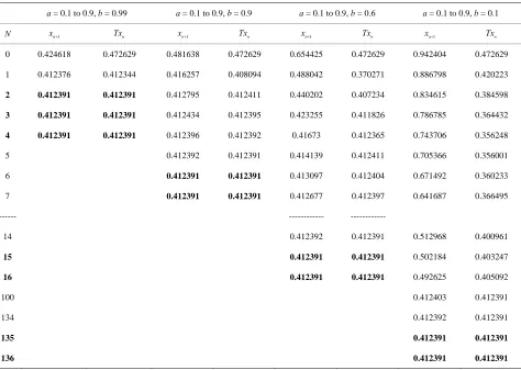
Table 2. Modified Ishikawa for

p x .

1

 

a = 0.1 to 0.9, b = 0.99 a = 0.1 to 0.9, b = 0.9 a = 0.1 to 0.9, b = 0.6 a = 0.1 to 0.9, b = 0.1

N xn1 Txn xn1 Txn xn1 Txn xn1 Txn

0 0.424618 0.472629 0.481638 0.472629 0.654425 0.472629 0.942404 0.472629

1 0.412376 0.412344 0.416257 0.408094 0.488042 0.370271 0.886798 0.420223

2 0.412391 0.412391 0.412795 0.412411 0.440202 0.407234 0.834615 0.384598

3 0.412391 0.412391 0.412434 0.412395 0.423255 0.411826 0.786785 0.364432

4 0.412391 0.412391 0.412396 0.412392 0.41673 0.412365 0.743706 0.356248

5 0.412392 0.412391 0.414139 0.412411 0.705366 0.356001

6 0.412391 0.412391 0.413097 0.412404 0.671492 0.360233

7 0.412391 0.412391 0.412677 0.412397 0.641687 0.366495

--- --- ---

14 0.412392 0.412391 0.512968 0.400961

15 0.412391 0.412391 0.502184 0.403247

16 0.412391 0.412391 0.492625 0.405092

100 0.412403 0.412391

134 0.412392 0.412391

135 0.412391 0.412391

[image:4.595.63.537.105.442.2]

136 0.412391 0.412391

Table 3. Simple Agarwal

et al. for

p x .

₁

 

a = 0.2, b = 0.9999 a = 0.2, b = 0.9 a = 0.3, b = 0.6 a = 0.5, b = 0.5

0 0.0803358 0.0100502 0.0733136 0.0100502 0.090521 0.0100502 0.177931 0.0100502

1 0.566185 1.3298 0.644644 1.3602 0.727194 1.2868 0.583438 0.965599

2 0.291318 0.20707 0.222863 0.134597 0.177672 0.0772623 0.323279 0.189489

25 0.412721 0.413097 0.418074 0.423399 0.420618 0.428339 0.412391 0.412392

26 0.412135 0.411843 0.407474 0.403035 0.405294 0.398897 0.412391 0.412391

27 0.412591 0.412817 0.416645 0.42061 0.418546 0.424292 0.412391 0.412391

55 0.412391 0.412392 0.412465 0.412533 0.412498 0.412596

56 0.412391 0.412391 0.412327 0.412269 0.412299 0.412214

95 0.412391 0.412392 0.412391 0.412392

96 0.412391 0.412391 0.412391 0.412391

97 0.412391 0.412392

(5)

[image:5.595.56.540.243.485.2]

Table 4. Modified Agarwal

et al. for

p x .

1

 

a = 0.9, b = 0.99 a = 0.1, b = 0.9 a = 0.3, b = 0.6 a = 0.9, b = 0.1

0 0.408091 0.472629 0.428901 0.472629 0.408937 0.472629 0.465458 0.472629

1 0.412381 0.412331 0.412289 0.412252 0.412356 0.412346 0.410188 0.409941

2 0.412391 0.412391 0.41239 0.41239 0.412391 0.412391 0.412368 0.412365

3 0.412391 0.412391 0.412391 0.412391 0.412391 0.412391 0.412391 0.412391

4 0.412391 0.412391 0.412391 0.412391 0.412391 0.412391 0.412391 0.412391

Table 5. Simple SP for

p x .

₁

 

a = 0.1, b = 0.1, c = 0.999 a = 0.1, b = 0.1, c = 0.9 a = 0.5, b = 0.5, c = 0.5 a = 0.1, b = 0.1, c = 0.1

0 0.0736477 0.0100502 0.139578 0.0100502 0.416514 0.0100502 0.667545 0.0100502

1 0.701496 1.35874 0.616499 1.09662 0.412245 0.405588 0.531266 0.116866

2 0.182726 0.0931953 0.271814 0.158438 0.412396 0.412634 0.463428 0.245717

3 0.617407 0.950211 0.519974 0.699365 0.412391 0.412382 0.433328 0.333637

4 0.242048 0.157633 0.334615 0.259135 0.412391 0.412391 0.420799 0.378667

5 0.566158 0.776228 0.471698 0.556962 0.412391 0.412391 0.415737 0.398604

--- --- --- --- --- ---

16 0.371841 0.341091 0.409891 0.406887 0.412391 0.412391

17 0.448911 0.483766 0.41427 0.416556 0.412391 0.412391

--- ---- ---- --- --- --- --- --- ---

50 0.41149 0.41072 0.412391 0.412391

51 0.413197 0.413889 0.412391 0.412391

--- --- --- --- --- ---- --- --- ---

126 0.412391 0.412391

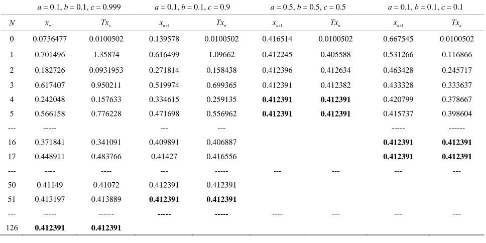
Table 6. Modified SP for

p x .

₁

 

a = 0.9, b = 0.9, c = 0.9999 a = 0.9, b = 0.9, c = 0.9 a = 0.2, b = 0.9, c = 0.1 a = 0.1, b = 0.1, c = 0.1

0 0.412399 0.472629 0.412496 0.472629 0.436509 0.472629 0.844335 0.472629

1 0.412391 0.412391 0.412391 0.412392 0.413946 0.411994 0.712973 0.367256

2 0.412391 0.412391 0.412391 0.412391 0.412512 0.412403 0.618933 0.359118

3 0.412391 0.412391 0.412391 0.412391 0.412401 0.412392 0.55555 0.37889

4 0.412391 0.412391 0.412391 0.412391 0.412392 0.412391 0.512865 0.394474

5 0.412391 0.412391 0.483669 0.403265

6 0.412391 0.412391 0.463373 0.407829

--- --- --- --- --- --- ---

---- --- ---

43 0.412392 0.412391

44 0.412392 0.412391

45 0.412391 0.412391

[image:5.595.59.540.510.732.2]

(6)

[image:6.595.57.539.107.427.2]

Table 7. Simple Noor for

p x .

1

 

a = 0.3, b = 0.3, c = 0.5 a = 0.3, b = 0.5, c = 0.7 a = 0.5, b = 0.7, c = 0.9 a = 0.5, b = 0.7, c = 0.9

0 0.506337 0.0100502 0.449615 0.0100502 0.331926 0.0100502 0.381042 0.0100502

1 0.417997 0.275966 0.410239 0.353812 0.506867 0.562555 0.442088 0.466838

2 0.412427 0.40316 0.41258 0.415975 0.34732 0.275298 0.389512 0.365152

3 0.412391 0.412331 0.412375 0.412077 0.485348 0.531107 0.433466 0.451642

5 0.412391 0.412391 0.412391 0.412389 0.470593 0.508772 0.395663 0.378452

6 0.412391 0.412391 0.412391 0.412391 0.367544 0.323489 0.427488 0.440836

7 0.412391 0.412391 0.459703 0.491825 0.400159 0.38787

75 0.412391 0.412392

76 0.412391 0.412391

155 0.412391 0.412392

156 0.412391 0.412391

157 0.412391 0.412391

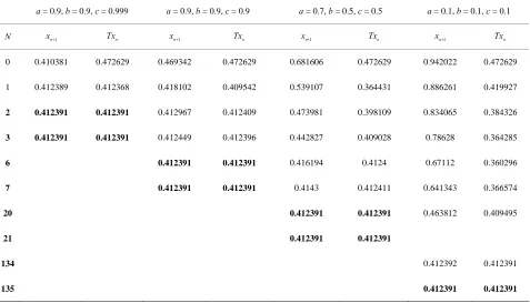
Table 8. Modified Noor for

p x .

1

 

a = 0.9, b = 0.9, c = 0.999 a = 0.9, b = 0.9, c = 0.9 a = 0.7, b = 0.5, c = 0.5 a = 0.1, b = 0.1, c = 0.1

0 0.410381 0.472629 0.469342 0.472629 0.681606 0.472629 0.942022 0.472629

1 0.412389 0.412368 0.418102 0.409542 0.539107 0.364431 0.886261 0.419927

2 0.412391 0.412391 0.412967 0.412409 0.473981 0.398109 0.834065 0.384326

3 0.412391 0.412391 0.412449 0.412396 0.442827 0.409028 0.78628 0.364285

6 0.412391 0.412391 0.416194 0.4124 0.67112 0.360296

7 0.412391 0.412391 0.4143 0.412411 0.641343 0.366574

20 0.412391 0.412391 0.463812 0.409495

21 0.412391 0.412391

134 0.412392 0.412391

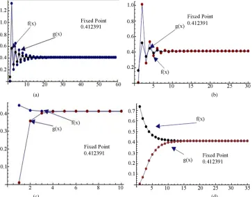
[image:6.595.62.539.462.735.2]

(7)

(a) (b)

[image:7.595.117.480.85.368.2]

(c) (d)

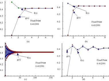
Figure 1. Graphical observations of simple Ishikawa iteration for

p x

₁

 

. Here (a)-(d) show the graph for Table 1. The

merg-ing point with value 0.412391 is fixed point.

[image:7.595.108.490.420.703.2]

(8)

Figure 3. Graphical observations of simple Agarwal

et al. iteration for

p x

₁

 

. Here (a)-(d) show the graph for Table 3. The

merging point with value 0.412391 is fixed point.

Figure 4. Graphical observations of new modified Agarwal

et al. iteration for

p x

1

 

. Here (a)-(d) show the graph for Table 4.

(9)

Figure 5. Graphical observations of simple SP iteration for

p x

₁

 

. Here Here (a)-(d) show the graph for Table 5. The

merg-ing point with value 0.412391 is fixed point.

Figure 6. Graphical observations of new modified SP iteration for

p x

1

 

. Here (a)-(d) show the graph for Table 6. The

(10)

[image:10.595.108.488.87.370.2]

Figure 7. Graphical observations of simple Noor iteration for

p x

₁

 

. Here (a)-(d) show the graph for Table 7. The merging

point with value 0 .412391 is fixed point.

Figure 8. Graphical observations of new modified Noor iteration for

p x

1

 

. Here (a)-(d) show the graph for Table 8. The

[image:10.595.85.518.424.691.2]

(11)

Table 9. Simple Ishikawa for

p

2

 

x .

a = 0.9, b = 0.999 a = 0.1, b = 0.9 a = 0.3, b = 0.5 a = 0.1, b = 0.1

0 0.340948 0.342793 0.343325 0.342793 0.346084 0.342793 0.349258 0.342793

1 0.340071 0.340243 0.341078 0.340895 0.343689 0.341668 0.348571 0.342578

2 0.339989 0.340005 0.340338 0.340278 0.342231 0.340996 0.347934 0.342379

3 0.339982 0.339983 0.340097 0.340078 0.341345 0.340593 0.347344 0.342195

6 0.339981 0.339981 0.339985 0.339984 0.340284 0.340116 0.345821 0.341726

7 0.339981 0.339981 0.339982 0.339982 0.340164 0.340063 0.345386 0.341593

9 0.339981 0.339981 0.340048 0.340011 0.344611 0.341357

10 0.339981 0.339981 0.340022 0.339999 0.344266 0.341253

18 0.339982 0.339981 0.342284 0.340659

20 0.339981 0.339981 0.341952 0.340561

21 0.339981 0.339981 0.341805 0.340517

127 0.339982 0.339981

128 0.339981 0.339981

[image:11.595.53.539.108.333.2]

129 0.339981 0.339981

Table 10. Modified Ishikawa for

p

₂

 

x .

a = 0.9, b = 0.9999 a = 0.1, b = 0.9 a = 0.3, b = 0.6 a = 0.1, b = 0.1

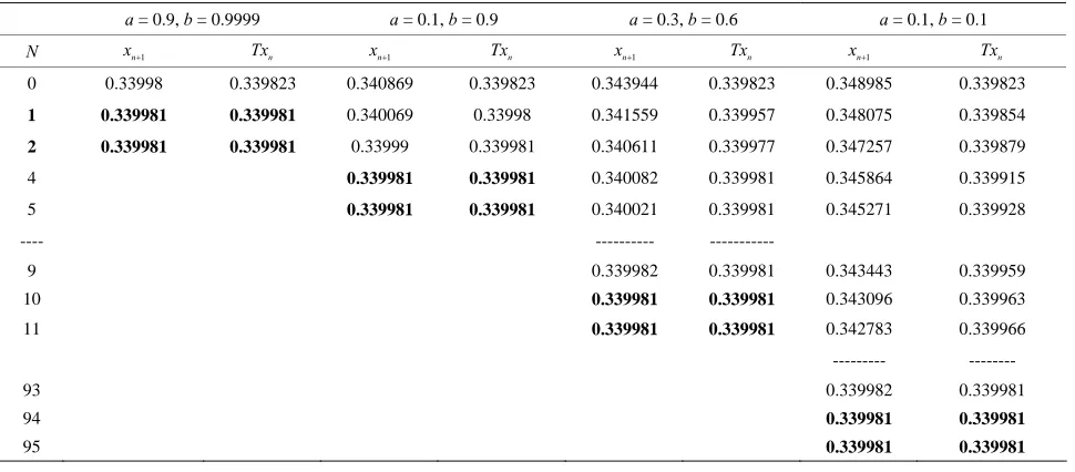
0 0.33998 0.339823 0.340869 0.339823 0.343944 0.339823 0.348985 0.339823

1 0.339981 0.339981 0.340069 0.33998 0.341559 0.339957 0.348075 0.339854

2 0.339981 0.339981 0.33999 0.339981 0.340611 0.339977 0.347257 0.339879

4 0.339981 0.339981 0.340082 0.339981 0.345864 0.339915

5 0.339981 0.339981 0.340021 0.339981 0.345271 0.339928

---- --- ---

9 0.339982 0.339981 0.343443 0.339959

10 0.339981 0.339981 0.343096 0.339963

11 0.339981 0.339981 0.342783 0.339966

--- ---

93 0.339982 0.339981

94 0.339981 0.339981

95 0.339981 0.339981

Table 11. Simple Agarwal

et al. for

p

₂

 

x .

a = 0.9, b = 0.99999, a = 0.1, b = 0.9 a = 0.3, b = 0.5 a = 0.1, b = 0.1

0 0.340949 0.342793 0.342605 0.342793 0.342481 0.342793 0.342772 0.342793 1 0.340071 0.340243 0.340649 0.340696 0.340587 0.340662 0.340737 0.340742 2 0.339989 0.340005 0.34015 0.340162 0.340127 0.340145 0.340184 0.340185

5 0.339981 0.339981 0.339984 0.339984 0.339983 0.339983 0.339985 0.339985

6 0.339981 0.339981 0.339982 0.339982 0.339982 0.339982 0.339982 0.339982

7 0.339981 0.339981 0.339981 0.339981 0.339981 0.339981 0.339981 0.339981

[image:11.595.57.542.364.577.2]

(12)

[image:12.595.56.539.237.473.2]

Table 12. Modified Aggarwal

et al. for

p

2

 

x .

a = 0.99999, b = 0.999 a = 0.1, b = 0.9 a = 0.1, b = 0.1 a = 0.1, b = 0.5

0 0.339981 0.339823 0.339851 0.339823 0.339827 0.339823 0.339839 0.339823

1 0.339981 0.339981 0.339981 0.339981 0.339981 0.339981 0.339981 0.339981

2 0.339981 0.339981 0.339981 0.339981 0.339981 0.339981 0.339981 0.339981

Table 13. Simple SP for

p

₂

 

x .

a = 0.9, b = 0.9, c = 0.999 a = 0.1, b = 0.1, c = 0.9 a = 0.3, b = 0.5, c = 0.7 a = 0.1, b = 0.1, c = 0.1

0 0.340313 0.342793 0.343012 0.342793 0.342455 0.342793 0.347988 0.342793

1 0.339992 0.340071 0.340881 0.340808 0.340583 0.340655 0.346375 0.342211

2 0.339981 0.339984 0.340247 0.340225 0.340127 0.340144 0.345085 0.34175

3 0.339981 0.339981 0.340059 0.340053 0.340016 0.34002 0.344053 0.341386

4 0.339981 0.339981 0.340004 0.340002 0.33999 0.339991 0.343229 0.341097

-- -- --- --- ---- --- --- --- ---

8 0.339981 0.339981 0.339981 0.339981 0.341292 0.340428

9 0.339981 0.339981 0.339981 0.339981 0.341026 0.340337

-- -- --- --- ---- --- --- --- ---

44 0.339981 0.339981

45 0.339981 0.339981

Table 14. Modified SP for

p

2

 

x .

a = 0.9, b = 0.9, c = 0.999 a = 0.1, b = 0.1, c = 0.9 a = 0.3, b = 0.5, c = 0.7 a = 0.1, b = 0.1, c = 0.1

0 0.340066 0.339823 0.34807 0.339823 0.343427 0.339823 0.34807 0.339823

1 0.339982 0.339981 0.346515 0.339879 0.34118 0.339963 0.346515 0.339879

2 0.339981 0.339981 0.345263 0.339915 0.3404 0.339979 0.345263 0.339915

3 0.339981 0.339981 0.344252 0.339938 0.340128 0.339981 0.344252 0.339938

-- -- --- --- ---- --- --- --- ---

8 0.341463 0.339976 0.339982 0.339981 0.341463 0.339976

9 0.341181 0.339978 0.339981 0.339981 0.341181 0.339978

10 0.340953 0.339979 0.339981 0.339981 0.340953 0.339979

-- -- --- --- ---- --- --- --- ---

46 0.339982 0.339981 0.339982 0.339981

47 0.339981 0.339981 0.339981 0.339981

[image:12.595.56.543.510.730.2]

(13)

[image:13.595.63.536.105.447.2]

Table 15. Simple Noor for

p

2

 

x .

a = 0.9, b = 0.9, c = 0.999 a = 0.1, b = 0.1, c = 0.9 a = 0.3, b = 0.5, c = 0.7 a = 0.1, b = 0.1, c = 0.1

0 0.340491 0.342793 0.34332 0.342793 0.344161 0.342793 0.349258 0.342793

1 0.340006 0.340119 0.341074 0.340894 0.341717 0.341127 0.34857 0.342577

2 0.339982 0.339988 0.340337 0.340277 0.3407 0.340452 0.347932 0.342378

3 0.339981 0.339981 0.340097 0.340077 0.340279 0.340176 0.347342 0.342195

4 0.339981 0.339981 0.340019 0.340012 0.340104 0.340061 0.346794 0.342025

5 0.339981 0.339981 0.339993 0.339991 0.340032 0.340014 0.346288 0.341869

6 0.339985 0.339984 0.340002 0.339995 0.345818 0.341725

7 0.339982 0.339982 0.33999 0.339987 0.345383 0.341592

8 0.339981 0.339981 0.339985 0.339983 0.344981 0.34147

9 0.339981 0.339981 0.339983 0.339982 0.344608 0.341357

10 0.339982 0.339981 0.344263 0.341252

11 0.339981 0.339981 0.343943 0.341156

12 0.339981 0.339981 0.343647 0.341067

13 0.339981 0.339981 0.343373 0.340984

-- -- --- --- ---- --- --- --- ---

127 0.339982 0.339981

128 0.339981 0.339981

129 0.339981 0.339981

Table 16. Modified Noor for

p

₂

 

x .

a = 0.9, b = 0.9, c = 0.999 a = 0.1, b = 0.1, c = 0.9 a = 0.3, b = 0.5, c = 0.7 a = 0.1, b = 0.1, c = 0.1

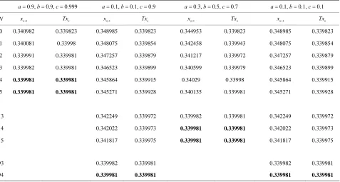
0 0.340982 0.339823 0.348985 0.339823 0.344953 0.339823 0.348985 0.339823

1 0.340081 0.33998 0.348075 0.339854 0.342458 0.339943 0.348075 0.339854

2 0.339991 0.339981 0.347257 0.339879 0.341217 0.339972 0.347257 0.339879

3 0.339982 0.339981 0.346523 0.339899 0.340599 0.339979 0.346523 0.339899

4 0.339981 0.339981 0.345864 0.339915 0.34029 0.33998 0.345864 0.339915

5 0.339981 0.339981 0.345271 0.339928 0.340135 0.339981 0.345271 0.339928

13 0.342249 0.339972 0.339982 0.339981 0.342249 0.339972

14 0.342022 0.339973 0.339981 0.339981 0.342022 0.339973

15 0.341817 0.339975 0.339981 0.339981 0.341817 0.339975

93 0.339982 0.339981 0.339982 0.339981

[image:13.595.62.539.482.737.2]

(14)

[image:14.595.104.498.85.368.2]

Figure 9. Graphical observations for simple Ishikawa iteration for

p

₂

 

x . Here (a)-(d) show the graph for Table 9. The

merging point with value 0.33981 is fixed point.

[image:14.595.102.494.415.697.2]

(15)

[image:15.595.96.504.89.366.2]

Figure 11. Graphical observations for simple Agarwal iteration for

p

2

 

x . Here (a)-(b) show the graph for Table 11. The

merging point with value 0.33981 is fixed point.

[image:15.595.105.492.409.701.2]

(16)

[image:16.595.110.492.85.373.2]

Figure 13. Graphical observations for simple SP iteration for

p

₂

 

x . Here (a)-(b) show the graph for Table 13. The merging

point with value 0.33981 is fixed point.

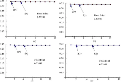
[image:16.595.96.498.420.703.2]

(17)

[image:17.595.103.502.82.366.2]

Figure 15. Graphical observations for simple Noor iteration for

p

₂

 

x . Here (a)-(b) show the graph for Table 15. The

merg-ing point with value 0.33981 is fixed point.

[image:17.595.94.506.410.700.2]

(18)

[image:18.595.55.538.121.364.2]

4. Observations

Table 17. Simple-Ishikawa for

p x .

1

 

a/b 0.001 0.01 0.1 0.2 0.3 0.4 0.5 0.6 0.7 0.8 0.9 0.99 0.999 0.9999

0.001 5513 546 49 16 11 6 13 24 86 not not not not Not

0.01 5590 554 50 22 12 7 12 24 72 not not not not not

0.1 6503 645 59 26 15 9 8 12 24 53 3476 not not Not

0.2 7994 794 74 34 20 13 8 6 11 17 28 50 54 54

0.3 10455 1040 99 46 29 20 14 10 7 7 9 13 13 13

0.4 15285 1523 147 70 45 32 24 18 14 12 10 9 9 9

0.5 29149 2909 285 140 91 66 52 42 34 28 21 23 22 22

0.6 916911 91684 9161 4577 3048 2284 1826 1520 1301 1137 1009 916 907 906

0.7 not not not not not not not not not not not not not not

Table 18. Modified-Ishikawa for

p x .

1

 

a/b 0.001 0.01 0.1 0.2 0.3 0.4 0.5 0.6 0.7 0.8 0.9 0.99 0.999 0.9999

0.001 14030 1397 134 63 40 28 21 16 12 9 6 4 4 4

0.01 14032 1397 134 63 40 28 21 16 12 9 6 4 4 4

0.1 14056 1400 134 63 40 28 21 16 12 9 6 5 4 4

0.2 14086 1403 134 64 40 28 21 16 12 9 5 5 4 4

0.3 14119 1406 134 64 40 28 21 16 12 9 5 5 4 4

0.4 14152 1409 135 64 40 28 21 16 12 9 6 4 4 4

0.5 14181 1412 135 64 40 28 21 16 12 9 6 4 4 4

0.6 14204 1414 135 64 40 28 21 16 12 9 6 4 4 4

0.7 14220 1416 136 64 40 28 21 16 12 9 7 4 4 4

0.8 14224 1416 136 64 40 28 21 16 12 9 7 3 3 3

0.9 14216 1416 135 64 40 28 21 16 12 9 7 4 3 3

0.99 14197 1414 135 64 40 28 21 16 12 9 7 4 3 3

[image:18.595.61.541.394.732.2]

0.999 14195 1414 135 64 40 28 21 16 12 9 7 4 3 3

Table 19. Simple-Ishikawa

for

p x .

1

 

a/b 0.001 0.01 0.1 0.2 0.3 0.4 0.5 0.6 0.7 0.8 0.9 0.99 0.999 0.9999

0.001 13701 1366 132 65 41 29 23 18 15 12 10 8 8 8

0.01 13667 1363 132 64 41 29 22 18 14 12 10 8 8 8

(19)

Continued

0.2 12998 1296 125 60 39 28 21 17 13 11 9 8 7 7

0.3 12671 1263 122 59 38 27 20 16 13 11 9 7 7 7

0.4 12360 1232 119 57 36 26 20 16 12 10 8 7 7 7

0.5 12066 1203 116 56 36 25 19 15 12 10 8 7 6 6

0.6 11785 1174 113 54 35 25 19 15 12 9 8 6 6 6

0.7 11516 1148 110 53 34 24 18 14 11 9 7 6 6 6

0.8 11260 1122 108 52 33 23 18 14 11 8 7 6 6 5

0.9 11015 1096 106 50 32 23 17 13 10 8 7 5 5 5

0.99 10803 1076 104 49 31 22 17 13 10 8 6 5 5 5

[image:19.595.55.541.97.256.2]

0.999 10783 1074 103 49 31 22 17 13 10 8 6 5 5 5

Table 20. Modified-Ishikawa

for

p

₂

 

x .

a/b 0.001 0.01 0.1 0.2 0.3 0.4 0.5 0.6 0.7 0.8 0.9 0.99 0.999 0.9999

0.001 9977 994 95 45 28 20 15 11 9 7 5 3 2 2

0.01 9977 994 95 45 28 20 15 11 9 7 5 2 2 2

0.1 9980 994 95 45 28 20 15 11 9 7 5 2 2 2

0.2 9983 994 95 45 28 20 15 11 9 7 5 2 2 2

0.3 9985 994 95 45 28 20 15 11 9 7 5 2 2 2

0.4 9987 995 95 45 29 20 15 11 9 7 5 3 2 2

0.5 9988 995 95 45 29 20 15 11 9 7 5 3 2 2

0.6 9990 995 95 45 29 20 15 11 9 7 5 3 2 2

0.7 9991 995 95 45 29 20 15 11 9 7 5 3 2 2

0.8 9992 995 95 45 29 20 15 11 9 7 5 3 2 2

0.9 9992 995 95 45 29 20 15 11 9 7 5 3 2 2

0.99 9992 995 95 45 29 20 15 11 9 7 5 3 2 2

[image:19.595.55.540.528.733.2]

0.999 9992 995 95 45 29 20 15 11 9 7 5 3 2 2

Table 21. Simple-Agarwal for

p x .

1

 

a/b 0.001 0.01 0.1 0.2 0.3 0.4 0.5 0.6 0.7 0.8 0.9 0.99 0.999 0.9999

0.001 not not not not not not Not not not not not not not not

0.2 not not not not not not Not not not 291 97 59 57 57

0.3 not not not not not not 5475 101 47 29 19 14 14 14

0.4 not not not not not 307 59 29 19 11 8 9 10 10

0.5 not not not not not 59 27 15 9 9 15 23 24 24

0.6 not not not not 101 29 15 7 10 17 37 288 741 885

0.7 not not not not 47 18 9 8 20 62 not not not not

0.8 not not not 287 29 11 8 19 68 not not not not not

0.9 not not not 95 17 7 15 53 not not not not not not

0.99 not not not 55 14 10 33 not not not not not not not

(20)

[image:20.595.54.539.106.329.2]

Table 22. Modified-Agarwal for

p x .

1

 

a/b 0.001 0.01 0.1 0.2 0.3 0.4 0.5 0.6 0.7 0.8 0.9 0.99 0.999 0.9999

0.001 4 4 4 4 4 4 4 4 4 4 4 4 4 4

0.01 4 4 4 4 4 4 4 4 4 4 4 4 4 4

0.1 4 4 4 4 4 4 4 4 4 4 4 4 4 4

0.2 4 4 4 4 4 4 4 4 4 4 4 4 4 4

0.3 4 4 4 4 4 4 4 4 4 4 4 4 4 4

0.4 4 4 4 4 4 4 4 4 4 4 4 4 4 4

0.5 4 4 4 4 4 4 4 4 4 4 4 4 4 4

0.6 4 4 4 4 4 4 4 4 4 4 4 4 4 4

0.7 4 4 4 4 4 4 4 4 4 4 4 4 4 4

0.8 4 4 4 4 4 4 4 4 4 3 3 3 3 3

0.9 4 4 4 4 4 4 4 3 3 3 3 3 3 3

0.99 4 4 4 4 4 4 4 3 3 3 3 3 3 3

[image:20.595.55.539.359.564.2]

0.999 4 4 4 4 4 4 4 3 3 3 3 3 3 3

Table 23. Simple-Agarwal for

p

₂

 

x .

a/b 0.001 0.01 0.1 0.2 0.3 0.4 0.5 0.6 0.7 0.8 0.9 0.99 0.999 0.9999

0.001 8 8 8 8 8 8 8 8 8 8 8 8 8 8

0.01 8 8 8 8 8 8 8 8 8 8 8 8 8 8

0.1 8 8 8 8 8 8 8 8 8 8 8 8 8 8

0.2 8 8 8 8 8 8 8 8 8 8 8 8 7 7

0.3 8 8 8 8 8 8 8 8 7 7 7 7 7 7

0.4 8 8 8 8 8 8 7 7 7 7 7 7 7 7

0.5 8 8 8 8 8 7 7 7 7 7 7 6 6 6

0.6 8 8 8 8 8 7 7 7 7 7 6 6 6 6

0.7 8 8 8 8 7 7 7 7 6 6 6 6 6 6

0.8 8 8 8 8 7 7 7 7 6 6 6 6 5 5

0.9 8 8 8 8 7 7 7 6 6 6 5 5 5 5

0.99 8 8 8 7 7 7 6 6 6 6 5 5 5 5

0.999 8 8 8 7 7 7 6 6 6 5 5 5 5 5

Table 24. Modified-Agarwal

for

p

₂

 

x .

a/b 0.001 0.01 0.1 0.2 0.3 0.4 0.5 0.6 0.7 0.8 0.9 0.99 0.999 0.9999

0.001 2 2 2 2 2 2 2 2 2 2 2 2 2 2

0.01 2 2 2 2 2 2 2 2 2 2 2 2 2 2

0.1 2 2 2 2 2 2 2 2 2 2 2 2 2 2

0.2 2 2 2 2 2 2 2 2 2 2 2 2 2 2

0.3 2 2 2 2 2 2 2 2 2 2 2 2 2 2

0.4 2 2 2 2 2 2 2 2 2 2 2 2 2 2

0.5 2 2 2 2 2 2 2 2 2 2 2 2 2 2

[image:20.595.55.539.590.732.2]

(21)

Continued

0.7 2 2 2 2 2 2 2 2 2 2 2 2 2 2

0.8 2 2 2 2 2 2 2 2 2 2 2 2 2 2

0.9 2 2 2 2 2 2 2 2 2 2 2 2 2 2

0.99 2 2 2 2 2 2 2 2 2 2 2 2 2 2

0.999 2 2 2 2 2 2 2 2 2 2 2 2 2 2

We have noted the converging step of different

itera-tions in tabular form and compare the conversing step for

different value of a, b, c. Now by comparative analysis

we noted that

1) For

p x

1

 

.1

0.8 , simple Ishikawa do not converge for

,

and

,

but

new modified Ishikawa converges for all values of a and

b converges faster than Ishikawa iteration for corre-

sponding values of a, b. Also it converges at lesser step

as a and b both approaches one but not so in case of sim-

ple Ishikawa as observe from

Tables 17

and

18 . Simi-

larly if we compare the both iterations for

0  

a

0  

b

1

0.6  

a

1

0  

b

1  

2

p x

as

observed from

Tables 19

and

20 that as we increase val-

ues of a and b simultaneously than converging step de-

creases for both iterations but modified Ishikawa itera-

tion converges at lesser step for

p x

2

 

.

2) As observed from

Tables 21

and

22 for

p

1

 

x

simple Agarwal

et al.

do not converge for all values of a

and b it converges for



a



0.2, 0.8

 

b

1 

0.4, 0.5, 0.4

a





b

,



a



0.3, 0.5

 

b

1 





1 



a



0.6, 0.3

 

b

1 

,



a



0.7, 0.3

 

b

0.8 

,



0.8  

a

1, 0.2



b



0 .5



but modified new Agarwal

et al.

iteration converges at

lesser step for all values of a, b. For

both itera-

tions converge for all values of a and b but modified

it-eration converges faster than simple itit-eration

 

2

p x

3) The simple SP iteration converges at lesser step for

when

a

= 1/2,

b

= 1/2,

c

= 1/2 as we increases a

and b the step of convergence increases. But do not con-

verge if a and b approaches to one whereas modified new

SP iteration converges for all values of a, b, c and at

lesser step than simple SP. For

both iteration

converges for all values of a, b and c but modified new

SP converge faster than Simple SP iteration.

 

1

p x

 

2

p x

4) For simple Noor and modified new Noor iteration

result is same as for SP and modified new SP iterations.

5. Conclusion

By the observation formed from the program and graph

drawn in C

++

and Mathematica for

p x

1

 

and

p x

2

 

polynomial, we conclude that the modified Ishikawa,

Agarwal

et al.

, SP, Noor are faster than simple Ishikawa,

Agarwal

et al.

, SP, Noor; but if we compare modified

Ishikawa, Agarwal

et al.

, SP, Noor with decreasing order

of rate of convergence of modified Agarwal

et al.

, SP,

Noor, Ishikawa, modified new Agarwal

et al.

have con-

sistent rate of convergence. The graphs drawn are based

on data formed from C

++

program and plot the data in

mathematica to show the fixed point.

REFERENCES

[1]

J. Biazar and A. Amirteimoori, “An Improvement to the

Fixed Point Iterative Method,”

Applied Mathematics and

Computation

, Vol. 182, No. 1, 2006, pp. 567-571.

http://dx.doi.org/10.1016/j.amc.2006.04.019

[2]

B. Prasad and R. Sahni, “Convergence of Some General

Iterative Schemes,”

International Journal of Mathemati-

cal Analysis

, Vol. 5, No. 25, 2011, pp. 1237-1242.

[3]

S. Ishikawa, “Fixed Points by a New Iteration Method,”

Proceedings of the American Mathematical Society

, Vol.

44, No. 1, 1974, pp. 147-150.

http://dx.doi.org/10.1090/S0002-9939-1974-0336469-5

[4]

R. P. Agarwal, D. O’Regan and D. R. Sahu, “Iterative

Construction of Fixed Points of Nearly Asymptotically

Non-Expansive Mappings,”

Journal of Nonlinear and Con-

vex Analysis

, Vol. 8, No. 1, 2007, pp. 61-79.

[5]

M. A. Noor, “New Approximation Schemes for General

Variational Inequalities,”

Journal of Mathematical Analy-

sis and Applications

, Vol. 251, No. 1, 2000, pp. 217-229.

http://dx.doi.org/10.1006/jmaa.2000.7042

[6]

W. Phuengrattana and S. Suantai, “On the Rate of Con-

vergence of Mann, Ishikawa, Noor and SP Iterations for

Continuous Functions on an Arbitrary Interval,”

Journal

of Computational and Applied Mathematics

, Vol. 235, No.

9, 2011, pp. 3006-3014.

http://dx.doi.org/10.1016/j.cam.2010.12.022

[7]

E. Babolian and J. Biazar, “On the Order of Convergence

of Adomian Method,”

Applied Mathematics and Compu-

tation

, Vol. 130, No. 2-3, 2002, pp. 383-387.