Exposure at Default Model for Contingent Credit Line

Munich Personal RePEc Archive

Exposure at Default Model for

Contingent Credit Line

Bag, Pinaki

1 April 2010

Online at

https://mpra.ub.uni-muenchen.de/20387/

Exposure at Default Model for Contingent Credit Line

By

Pinaki Bag*a

* Disclaimer:The author is working with Union National Bank (Bank), Abu Dhabi, UAE. The views expressed in the article are personal and do not represent the views of the Bank and the Bank is not responsible towards any party for these views.

Abstract

In-spite of large volume of Contingent Credit Lines (CCL) in all commercial banks

paucity of Exposure at Default (EAD) models, unsuitability of external data and

inconsistent internal data with partial draw-down, has been a major challenge for risk

managers as well as regulators for managing CCL portfolios. Current paper is an

attempt to build an easy to implement, pragmatic and parsimonious yet accurate model

to determine exposure distribution of a CCL portfolio. Each of the credit line in a portfolio

is modeled as a portfolio of large number of option instrument which can be exercised

by the borrower determining the level of usage. Using an algorithm similar to basic

CreditRisk+ and Fourier Transforms we arrive at a portfolio level probability distribution

of usage.

JEL Classification: G20, G21, C13

I Introduction

Bank for International Settlement (BIS) in its Basel II guidelines1 _{describes capital}

as a function of Probability of Default (PD), Loss Given Default (LGD) and Exposure at

Default (EAD) with all playing an equally vital role, but a simple Google search on each

term returns 5.7 Million, 65 Thousand and 29 Thousand2 _{hits respectively. Google}

search may not be concrete enough to conclude but it does indicate the trends in terms

of importance given to each component by academicians and practitioners. Similar

assertions are made by Financial Services Authority (FSA)3

, UK regarding EAD models

as well.

Contingent Credit Lines (CCL) or Loan Commitments4 _{are contractual promises}

by the bank to specific obligors to lend up to specified limits on pre-determined rates

and terms. They are generally accompanied with different fees which must be paid over

the life of the commitment, and the material adverse change (MAC) clause which states

that bank may cancel the line if the credit quality deteriorates of the specific obligor.

According to Federal Deposit Insurance Corporation survey5 _{close to 80% of all}

commercial and industrial loans are done using commitment contracts and as of

1 Refer BCBS (2006) revised document on Basel II guideline

2 Searched on 24 Feb 2010 from www.google.com

3 Please refer EAD Expectation Note (2007)

4 Contingent Credit Line, Loan/Credit Commitment, Line of Credit has been used interchangeably in the paper

September 2009, the outstanding (unused) CCLs of U.S. firms were close to $1.9

trillion. Avery and Berger (1991) states that main reason for using credit commitment is

to provide flexibility during slowdown and as noted by Kanatas (1987) these can be

seen as hedging instruments. Hawkins (1982) comments that credit lines help

borrowers manage fluctuations in working capital but Sufi (2008) reports that firm with

low cash flow or high cash flow volatility rely more heavily on cash rather than credit

line.

Basel II guidelines calculate regulatory capital charge of contingent credit

commitments based on credit conversion factor (0% to 50%) and the Risk Weight (0%

to 100%). As noted by Hull (1989), credit conversion factor (CCF) for a small bank

underestimates the capital requirement as “fat tails” effect increases the capital

requirement proportionately more for off-balance sheet items. In its Advanced Internal

Rating Based (AIRB) methodology Basel II does allow banks to compute its own

estimates of CCF and henceforth its own estimate of Exposure at Default (EAD) for

CCL.

Apart from negligence of EAD models by consultants and academics leading to a

paucity of external data and models, other issues identified by FSA, has been scarcity

of usable data regarding draw-downs in each bank and unsuitability of external data.

When external data is available the suitability is always questioned as the estimates will

be strongly influenced by lender's behavior.

accurate model for estimation of exposure for CCL portfolio. Each CCL is modeled as

portfolio of options with the obligors which they can exercise with the bank at

pre-specified terms & conditions. Modeling the exercise of options as a Poisson process, a

stochastic distribution of exposure at different segment of portfolio level has been

constructed. A standard Fast Fourier Transform algorithm is used to convolute these

portfolio segments and generate the exposure probability distribution of the complete

portfolio.

This model with help from internal research of the bank can be used for the

estimation of EAD for banks as mandated by Basel II for CCL portfolios. Apart from

regulatory requirement, stochastic exposure distribution generated can form as an input

for different economic capital model and stress testing procedures to capture accurate

risk profile of the portfolio. This will also contribute in providing better insights in the

problem of managing liquidity risk for portfolio of CCL e.g. credit card portfolio or Home

Equity Line of Credit (HELC) portfolio.

In the following pages we will see in section II about past studies related to CCL,

section III will detail on how we can use options executions to link the draw-downs in a

portfolio, section IV provides an implementation with hypothetical portfolios and finally

section V concludes with potential future research areas and implications.

II CCL, Options & Partial Draw-down

first form an appropriate conversion factor is multiplied with the total limit (TL) of the

facility.

EAD=CF .TL ₍₁₎

In the second form an appropriate conversion factor (α)6

is multiplied with the

unused part of the limit (L) of the facility.

EAD=CurrentExposure+α ⋅L ₍₂₎

As shown by Moral (2006) both will yield same results for EAD except when full

utilization is in place. As discussed by Miu and Ozdemir (2008) Basel CCF is equivalent

to α in equation (2). We will use equation (2) for all our subsequent analysis. As current

exposure and L are known modeling α i.e. partial draw-down of the unused limit will give

us clear insight into the problem of EAD estimation of CCL.

Studies related to CCL are concentrated around pricing of CCL7 _{and level of}

partial draw-down in each credit line. In the current endeavor we will concentrate on

latter.

Thakor et al. (1981) utilize a put option8 _{approach to price the loan commitments}

and measure the sensitivity of these values to changes in interest rates. Partial

draw-down on CCL is explained through, interest elasticity of demand for borrowed funds and

6This is also referred as Loan Equivalent amount (LEQ) in many literatures.

7Pricing of CCL option theoretic approach has been used by Loukoianova et al. (2006), Chateau (1990), Chateau and Wu (2003).

bank customer relationship dynamics. A firm with infinite opportunities for investment

and no restriction on capital structure or leverage, the interest elasticity will be perfectly

elastic and vice-versa. Alternatively if we look into the bank customer relationship

framework, customer will try to minimize the expected cost of renewal of the line in next

year and opportunity loss of not utilizing the full facility this year when availing the line.

Kaplan and Zingales (1997) find that the un-drawn portion of credit lines

decreases when firms are more liquidity constrained. Gatev and Strahan (2003)9 _report

that partial draw-downs increase when the commercial paper - T bill rate spread rises.

Both of these studies indicate presence of interest incentive framework for partial

down which inspired Jones and Wu (2009) for using the same for modeling partial

draw-down. They models credit quality as a jump-diffusion process while partial draw-down

and pricing of CCL is done as a function of dynamic credit state. The proportion of the

credit line drawn is modeled as function of the difference between alternative

opportunity rate and the marginal cost of line borrowings. Opportunity rate is defined as

the rate of interest charged to the borrower if she borrows outside the purview of the

defined credit line. To incorporate linking of loan spread to the credit default swap

spread of the borrower, marginal cost of borrowing is defined as function of reference

rate, contractual spread over reference rate and proportion of the excess that is added

to current period loan. Apart from the interest rate differential, sensitivity of drawdown

with interest rate differential is included to model amount of partial draw-down. This

sensitivity is similar to the interest elasticity proposed by Thakor et al. (1981).

Both of the approach (Thakor et al. (1981) and Jones et al. (2009)) looks intuitive

and convincing but implementing the same in banks where most of the CCL are

extended to unrated obligors whose market spread may not be easily available, might

pose problems of parameterization. Some parameter like interest elasticity may be

affected by firm specific behavior as well as present macro economic variables. Another

approach of estimating usage of limits under continuous-time model where the credit

provider and the credit taker interact within a game-theoretic framework has been

attempted by Leippold et al (2003).

Attempts to directly estimate partial draw-down has also been undertaken in past.

Asarnow and James (1995) present partial draw-down estimates based on credit lines

issued by Citibank to publicly-rated North American firms over the five-year period from

1987 to 1992. They found a downward sloping of usage level from high rated obligors to

low rated obligors i.e. lower rated firms would have already consumed their credit lines

earlier than when it approaches default. Similar trend is also noted by Araten and

Jacobs (2001) where partial draw-down decreases as the firm approaches default. Their

estimates of partial draw-down is based on 1,021 observations (408 facilities of 399

borrowers) at a quarterly frequency in the period 1Q 1995 - 4Q 2000 for Chase

borrowers. They also report that level of usage has been affected by risk rating but not

by commitment size and borrower industry. Jacobs (2008) empirical study is based on

credit ratings over the period from 1985 to 2006. He finds that similar trends in terms of

usage and points out statistically significant affect of obligor profits in the level of usage.

Agarwal et. al. (2005) examined utilization of HELC in US market and confirms

that borrowers with deteriorating credit quality increase their utilization. Jiménez et al.

(2009) reports a credit line usage of different firms granted by banks in Spain between

1984 and 2005. The final dataset used consisted of 696,445 credit lines granted to

334,442 firms by 404 banks. They reported variety of factors such as commitment size;

collateralization and maturity of the CCLs affect the usage level. They also report a

statistically significant higher usage rate for firms that are defaulting at least 3 years

prior to default and the usage monotonically increases as the default approaches for

these firms.

Level of usage is mainly affected by two distinct forces, the lender might realize

the deteriorating credit quality of the borrower and cut back the limits thereby increasing

the utilization ratio or the borrower may actually use up the line before the lender

realizes deteriorating credit quality. As indicated by Qi (2009) with credit card usage in

US, borrowers are more active than lenders in this game of “race to default.” Martin and

Santomero (1997) analyzes the pricing of CCL from demand side of firms and show that

credit line usage depends on business growth potential of the firm as well as the

uncertainty involved in those investment opportunities. External macro economic

variables, size of credit line, collateralization etc. may also determine level of partial

III Partial Draw-down at Portfolio Level

To put ourselves on firmer basis lets define a bank B with a CCL portfolio of N

obligors each having one facility of CCL each. Each of these credit lines with the bank

can be used before the expiry of the contract. For obligor A with CCL size of LA we can

safely assume that A has infinite number of put options which she can choose to

exercise and the number of instrument she will exercise will decide the level of partial

draw-down. If she exercises all the puts, than she will have consumed her whole limit.

We assume she has n number of puts at her disposal, where n is sufficiently large. Also

size of each put can be given as

Q_A=LA

n (5)

So the amount of partial draw-down can be given as r X QA where r is the number

of puts exercised by A in the time frame of consideration. So the probability generating

function (PGF) of the option exercise can be defined as follows:

F_Az=Pr=0Z0+Pr=1Z1+Pr=2Z2+Pr=3Z3+Pr=4Z4. . . . .. ₍₆₎

Let’s assume expected usage of the CCL is αA so average number of puts used

by A is λ_A=αALA

Q_A (7)

Using a Poisson process of exercise of each option we have the PGF given by

F_Az=e

−λA

λ0

0! Z

0_e −λA

λ1

1! Z

1_e −λA

λ2

2! Z

2_{. . .}

= F_Az=e−λA

eλAZ

(8)

For all obligors, m (m<N) in the portfolio having put size equal to Q we have the

PGF for r number of puts being used and assuming independence of obligors in

exercising of each option

∏





∏

eλAZ

=e

∑ i=1 i=m

−λi∑

i=1 i=m λ

iZ ₍₉₎

Now lets assume the overall average usage in the portfolio is α and unused limits

in this portfolio of m obligor be Li hence we have

α=

∑

i=1

i=m

α_iL_i

∑

i=1

i=m

L_i

(10)

Let S_i=

∑

i=1

i=m

λ_i and as we have assumed all the size of put is Qi henceforth and let

β_i=

∑

i=1

i=m

S_i⋅Q_i so

S_i=

∑

i=1

i=m

λ_i=

∑

i=1

i=m

α_iL_i

Q_i = α Q_i⋅

∑

i=m

L_ihenceβ_i=α⋅

∑

i=1

i=m

L_i (11)

So the PGF of usage being equal to r X Q will be given by

F_Q1z=eZ−1S1_=e−S1

[





0

0! 





1

1! 





2

2! . . ..

]

Now for any real portfolio, Q will not be equal for all obligors. To simplify our

obligors in each sub-portfolio will have same size of put as Qi. Since in each

sub-portfolio Qi is same whenever there is exercise of 1 put there is usage of 1XQi and if

there is exercise of 2 puts there is usage of 2XQi so we can write:

P









So the PGF of the sub-portfolio usage can be written as:

F_QiZ=

∑

r=0 ∞

PUsage=r.Q_iZr.Qi=

∑

r=0 ∞

PUsage=rZr.Qi ₍₁₄₎

FQiz=

∑

∞

e−SiSi

r

r! Z

r.Qi

=e−Si

eSiZ

Q_i

(15)

Hence to find the usage distribution of the whole portfolio we must convolute

each of these portfolios. Hence form equation (11) for the whole portfolio with t

sub-portfolios PGF can be written as (assuming independence of each sub-portfolio):

_F

Qz=

∏

t

F_Q

iz=

∏

i=1

t

e−Si

eSiZ

Q_i

=e −∑

i=1 t

Si∑

i=1 t S iZ Q_i (16)

Now to determine the exposure distribution of the portfolio we can have from

Taylor’s theorem

PUsage=r.Q_i=1

r!

drF_Qz

dzr ∣Z=0 for r=0,1,2,… (17)

Let

W_r=1

r!

drF_QZ

dzr ∣Z=0=

1

r! dr−1 dzr−1

dF_QZ 

dz ∣Z=0 ₍₁₈₎

As

∑

i=1

t

W_r=1

r! dr−1

dzr−1FQZ. d

∑

i=1

t

S_iZQi

dz ∣z=0

(19)

By Lebinitz’s formula for nth _{order differentiation we can have:}

W_r=1

r!

∑

r−1

r−1_C

k.

dr−1−kF_QZ

dzr−1−k .

dk+1

∑

i=1

t

S_iZQi

dzk+1 ∣Z=0

(20)

If Qi=K+1 _{& Z =0 then}

d

k+1_

_∑

i=1

t

S_iZQi_

dzk+1 =k+1!Si

(21)

else if Q_i≠K+1 d

k+1_

_∑

i=1

t

S_iZQi_

dzk+1 =0

(22)

And we have from equation (18)

W_r−1−k= 1 r−1−k!

dr−1−kF_QZ

dZr−1−k ∣Z=0 (23)

Hence combining equation (20), (21), (22) and (23) at Z=0 we have

W_r=1

r! _k=Q

∑

i−1

r−1

r−1_C

k.k+1!Si.r−1−k!Wr−1−k∣Z=0 =

1

r _i;Q

∑

i≤r

Q_i.S_i.W_r−Q

i (24)

Hence from (24) and (10)

Wr=

1

r _i;Q

∑

i≤r

β_i.W_r−Q

i (25)

get the complete probability distribution of portfolio usage, starting fromW₀=

∑

i=1

t

S_i .

If we let Qi vary from 1 we will have exposure distribution from 1 $ as seen from

equation (3) Qi represents the size of each put.

Till now we have used a constant α for the whole portfolio, in reality we will have

a portfolio where α will be different for each segment of the portfolio depending upon

product type, and other factors etc. As noted in a survey10 _{banks generally prefer to use}

segment wise α for its EAD estimation. Hence after performing the computation till

equation 25 we will be left with probability distribution of usage for different segments of

the portfolio. To finally arrive at a portfolio level exposure distribution we will follow a

standard convolution procedure using Fourier Transforms.

For simplicity lets assume we have only two distinct segment of the CCL portfolio

and from (25) we can have two distinct vectors (F =f0,f1,…fl-1& G=g0,g1,….gm-1)

representing the probabilities of usage for each segment. Let R represent the vector

formed by convolution of F and G. To perform Fast Fourier Transform (FFT)11 _{we will}

pad each of the vector such that length of each vector is s, where s=>l+m and s is of the

form 2x _{where x is an integer. We know from convolution theorem that}

R=F G=Inverse FFT⊗ FFT F.FFT G (26)

Hence R will give us the overall portfolio usage probability distribution. The

procedure can easily be replicated if we have more than two segments in our portfolio.

10See RMA Survey (2004) on estimation of EAD & LGD

IV Numerical Experiment

For a typical CCL portfolio, ΣSi for the whole portfolio may be quite large and we

are trying to assign probability to each dollar of usage in the algorithm so it may finally

turn out to be daunting task to achieve the full distribution. For the calculation of

negative exponential of a very large number (ΣSi) for initiation of the calculation (as W0)

we will soon be confronted with precision issues under double-precision12 _{regime of}

most common software applications. Most applications including Matlab, Octave or

Microsoft Excel under default settings will approximate W0 as zero and as the

distribution depends on W0 for derivation of full distribution, the full distribution would be

evaluated incorrectly.

There may be many alternative to circumvent the problem in standard

applications. One solution to this problem may be use of libraries which can handle very

high precision calculation13_{. This may also require higher computational power in terms}

of hardware as well, the specification of which is beyond the scope of the current paper.

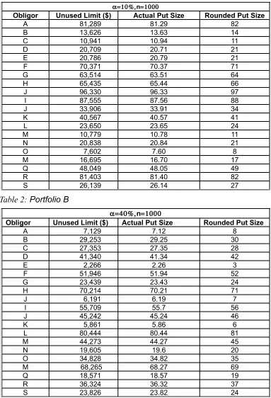
For illustration14 _{we have chosen two sample segments}15 _{of 20 obligors each with}

of α =10% and α = 40% respectively with limits16 _{of each obligor varying from $2,266 to}

$96,330. Each of the obligor limit is divided into 1,000 puts. The figure in appendix B

illustrates that the usage distribution of each segment and final convoluted portfolio; the

12For details see Monniaux (2008)

13 See http://gmplib.org/ for details

14 The calculations are done using Linux based Genius 1.0.7 as arbitrary precision calculator and Linux based Octave for FFT and final distribution evaluation.

15 Details of the portfolio presented in appendix A

descriptive statistics of each of the distributions are presented in table 3 of appendix B

for reference.

To explore the affect of choice of n in the exposure distribution we use first five

obligors of portfolio A. The results of the experiment are summarized in Table 3 in

appendix C. As noted the standard deviation of the usage distribution decreases as we

increase the number of puts used. This may be explained by the fact that we are

implicitly assuming a known value of α in our modeling i.e. a zero volatility of α and this

fact is becoming more prominent once we start increasing the number of puts (n) i.e.

more like real life scenario. The mean value remain relatively stable but the extreme

points converge towards the mean to produce a shrinkage in the distribution shape.

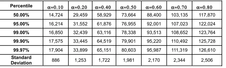
Another prime variable in the algorithm is the value set for α, we vary the value of

α to find its affect on the final distribution. The results of the same are summarized in

Table 4 in appendix C. For our 5 obligor portfolio we see increase in the usage level

also increase the volatility associated.

To incorporate volatility of α explicitly in the model we can also use a mixed

Poisson process where we chose different values of λ from an assumed distribution.

More commonly used mixture distribution has distribution of λ as Gamma distribution,

resulting in negative binomial; this has the advantage of analytically tractable two

parameter distribution. Similar combination17 _{can be used to incorporate volatility of} α

explicitly in each segment of the portfolio.

An argument against using any mixed distribution may be that this will induces a

second set of assumptions in our model and will require the banks to calculate usage

volatility of each segment. In the current model the volatility of the final distribution will

depend how spread out the expected usage is between each the segment. This may be

more pragmatic approach considering that it will have minimum data requirement at

portfolio-segment level and segmentation of the portfolio can be decided with internal

research and expert judgment on usage.

One of the segmentation possibilities of the portfolio may be based on

commitment fee18 _{and service fee}19_{. As shown by Thakor and Udell (1987) when the}

bank is uncertain about the level of partial draw-down, it may segregate borrowers by

keeping high commitment fees and low service fees in one contract and low

commitment fees and high service fees in other contract. Former would be attractive to

borrowers with higher probability of draw-down as they are more probable to pay a

service fee and more interested in having an active credit line, this will not be true for

borrowers who are less confident about draw-downs. Contract choice may not be

always that simple as discussed by Maksimovic (1990) it may also depend on structure

of the borrower’s industry, as in imperfect competition presence of predetermined rates

of financing in borrowers armory provides enhanced strategic position.

V Conclusion

This paper formulated a parsimonious model for estimation of exposure at

portfolio level for a typical CCL portfolio by modeling each CCL with a borrower as a

portfolio of option instruments. The exercise of each put has been modeled as standard

Poisson process where average usage (α) of CCL at the portfolio level is assumed to be

known. This value as indicated by Agarwal et. al. (2005), Qi (2009), Jiménez et al.

(2009) Gatev et al. (2006) etc. depends on change in credit quality, difference between

contractual rate and actual market rate and other factors. Both empirical research and

theory suggest a correlation between credit quality and usage of credit line. The

algorithm presented here can accommodate different values of α, to handle mentioned

correlation the portfolio may be segmented in terms of credit quality along with any

other criterion decided by the bank. Some of the methods of estimating α has been

outlined by Moral (2006) and similar research needs to done on the area of finding

expected usage at a given type of portfolio and as indicated earlier, they can work best

if the bank themselves does the research on internal data, as this will be highly

influenced by Bank’s behavior in catching early signs of deterioration in credit quality.

Further work may also be needed so that stable distribution parameters can be

determined which will not be affected by choice of number of puts used.

Most of the current credit risk model viz. JP Morgan’s CreditMetrics, KMV

Portfolio Manager, CSFB CreditRisk+20 _{has constant exposure as an input to calculate}

credit Value-at-Risk. Rosen and Marina (2002) describes that stochastic exposures

make a notable difference in credit economic capital calculation. Akkaya and Wagner

(2003) describe stochastic exposure in CreditRisk+ modeling framework. Stochastic

Exposure generated from the discussed model can be useful in improvement of credit

economic capital modeling for CCL portfolio.

Accurate exposure calculation is fundamental for liquidity risk management as

well, e.g. credit card portfolio or HELC where all the accounts has a un-drawn but

committed line pose a challenge to risk managers in terms of expected usage and

henceforth liquidity positions; the algorithm presented here may prove helpful in

providing meaningful insight into the problem.

The other implication of the algorithm is in the area of EAD estimation for Basel

II. As pointed out earlier compared to PD estimation, limited research has gone in

estimating EAD. This can provide a good starting point for the banks under AIRB

approach of Basel II. Finally this may also be used in terms of stress testing tool to

determine worst case liquidity scenarios for the portfolio. As we have the complete

distribution of the usage value we can get a good estimate of our worst case scenarios

from 99th

or 99.9th

percentile depending upon the risk appetite of the bank.

Further work needs to be done to improve the algorithm so as to use it in

standard software applications with minimized hardware requirements. This will greatly

Reference

[1] Agarwal, S., and Ambrose, B. “Credit lines and credit utilization.” Journal of Mon-ey, Credit and Banking 38(1) (2006): 1–22.

[2] Akkaya, N., Kurth, A. and Wagner, A. “Incorporating default correlations and severity variations” in M. Gundlach and F. Lehrbass [13]

[3] Araten, Michel and Michael Jacobs, Jr. “Loan Equivalents for Revolving Credits and Advised Lines.” The RMA Journal, (2001): 34-39.

[4] Asarnow, E. and Marker, E. “Historical Performance of the U.S. Corporate Loan Market: 1988-1993,” Commercial Lending Review, 10(2), (1995): 13-32.

[5] Avery, Robert B., and Alan N. Berger. “Loan Commitments and Bank Risk Expo-sure.” Journal of Banking and Finance 15, (1991):173–192

[6] Basel Committee of Banking Supervision, “Basel II: International convergence of capital measurement and capital standards: a revised framework.” Available at www.bis.org/publ/bcbs118.htm, 19 Nov. 2009.

[7] Board of Governors of the Federal Reserve System, (2009) “Survey of Terms of Business Lending.” Federal Reserve Board Statistical Releases, E.2 Available at http://www.federalreserve.gov/releases/e2/current/default.htm, 21 Nov. 2009

[8] Chateau, John Peter D and Jian Wu (2004) “Basle II Capital Adequacy: Comput-ing the 'Fair' Capital Charge for Loan Commitment 'True' Credit Risk.” EFMA 2004 Basel Meetings Paper. Available at SSRN: http://ssrn.com/abstract=497546

[9] Château., John-Peter D. "Valuation of ‘capped’ variable rate loan commitments" Journal of Banking & Finance Volume 14, Issue 4, (1990):717-728

[10] Credit Suisse, (1997). CreditRisk+: A Credit Risk Management Framework. Credit Suisse Financial Products. Available at www.csfb.com/creditrisk, 1997.

[11] Crouhy, M., D. Galai, and R. Mark. “A Comparative Analysis of Current Credit Risk Models.” Journal of Banking and Finance 24 (2000):59–118.

[12] Ergungor, Ozgur E., 2001, Theories of bank loan commitments: A literature re-view, Federal Reserve Bank of Cleveland Economic Review 37, 2-19.

[14] M. Gundlach and F. Lehrbass (eds.), CreditRisk+ in the Banking Industry, Springer-Verlag, Berlin, Heidelberg, 2004.

[15] D. Karlis and E. Xekalaki, “Mixed Poisson distributions,” International Statistical Review, vol. 73, no. 1, (2005):35–58

[16] Federal Deposit Insurance Corporation, Statistics on Banking, (2009) table RC-6 Available at http://www2.fdic.gov/SDI/main4.asp

[17] Financial Services Authority, UK. Comments on EAD models (2007). EAD Expec-tation Note. Available at http://www.fsa.gov.uk/pubs/international/ead_models.pdf

[18] Gatev, Evan and Philip Strahan, “Banks Advantage in Hedging Liquidity Risk: Theory and Evidence from the Commercial Paper Market.” Journal of Finance 61, (2006):867-892.

[19] Gordy, M. B., “A Comparative Anatomy of Credit Risk Models.” Journal of Banking and Finance 24 (2000):119–149.

[20] Hull, J., “Assessing Credit Risk in a Financial Institution’s Off-Balance Sheet Com-mitments.” Journal of Financial and Quantitative Analysis, 24(4), (1989): 489-501.

[21] Jacobs, M., Jr., “An Empirical Study of Exposure at Default,” Manuscript, Office of the Comptroller of the Currency, U.S. Department of the Treasury. (2008)

[22] Jimenez, Gabriel, Jose A. Lopez, and Jesus Saurina, “Empirical analysis of corpo-rate credit lines”, Working Paper, Banco de Espana and Federal Reserve Bank of San Francisco.(2008)

[23] Jones, Robert, Yan Wendy Wu Analyzing credit lines with fluctuating credit quality. Working Paper, The Bank of Canada - Simon Fraser University Conference on Financial Market Stability. (2009)

[24] Kanatas, George., ”Commercial Paper, Bank Reserve Requirements, and the In-formational Role of Loan Commitments.” Journal of Banking and Finance 11, (1987):425–448

[25] Kaplan, Steven and Luigi Zingales “Do Investment-Cash Flow Sensitivities Pro-vide Useful Measures of Financing Constraints?” Quarterly Journal of Economics 112, (1997):169-215.

[27] M. Leippold, S. Ebnoether, P. Vanini, “Optimal Credit Limit Management,” National Centre of Competence in Research Financial Valuation and Risk Management, Working Paper No. 72. (2003)

[28] Maksimovic, V. “Product Market Imperfections and Loan Commitments,” Journal of Finance, vol. 45 (1990), pp. 1641–54.

[29] Martin., J. Spencer and Anthony M. Santomero “Investment opportunities and cor-porate demand for lines of credit, ”Journal of Banking & Finance, Volume 21, Issue 10, (1997):1331-1350

[30] Melchiori, Mario R., “CreditRisk+ by Fast Fourier Transform,” YieldCurve, August 2004. Available at SSRN: http://ssrn.com/abstract=1122844

[31] Miu, P., and B. Ozdemir., Basel II Implementation: A Guide to Developing and Vali-dating a Compliant Internal Risk Rating System, McGraw-Hill Professional, (2008): 173.

[32] Moral, G., “EAD Estimates for Facilities with Explicit Limits” in Engelmann, B. and Rauhmeier, R., eds. The Basel II Risk Parameters: Estimation, Validation, and Stress Testing. New York: Springer, (2006):197-242.

[33] Qi, M., “Exposure at Default of Unsecured Credit Cards”, Credit Risk Analysis Di-vision, Office of the Comptroller of the Currency, 250 E St. SW, Washington, DC 20219; (2009)

[34] RMA – The Risk Management Association (2004) Industry Practices in Estimating EAD and LGD for Revolving Consumer Credits – Cards and Home Equity Lines of Credit. Available at http://www.rmahq.org/../RMA_EAD_LGD_Survey_Paper_FINAL.pdf

[35] Robertson, J., “The Computation of Aggregate Loss Distributions,” PCAS LXXIX, (1992): 57–133.

[36] Rosen, D., and M. Sidelnikova, “Understanding Stochastic Exposures and LGD’s in Portfolio Credit Risk”, Algo Research Quaterly, Vol. 5, N° 1, (2002):43-56.

[37] Sufi, Amir. “Bank Lines of Credit in Corporate Finance: An Empirical Analysis.” The Review of Financial Studies, Vol. 22, Issue 3, (2009):1057-1088

[38] Thakor, Anjan V., Hai Hong and Stuart I. Greenbaum, "Bank Loan Commitments and Interest Rate Volatility," Journal of Banking and Finance, Vol. 5, (1981):497-510.

Appendix A

Table 1: Portfolio A

α=10%,n=1000

Obligor Unused Limit ($) Actual Put Size Rounded Put Size

A 81,289 81.29 82

B 13,626 13.63 14

C 10,941 10.94 11

D 20,709 20.71 21

E 20,786 20.79 21

F 70,371 70.37 71

G 63,514 63.51 64

H 65,435 65.44 66

J 96,330 96.33 97

I 87,555 87.56 88

J 33,906 33.91 34

K 40,567 40.57 41

L 23,650 23.65 24

M 10,779 10.78 11

N 20,838 20.84 21

O 7,602 7.60 8

M 16,695 16.70 17

Q 48,049 48.05 49

R 81,403 81.40 82

S 26,139 26.14 27

Table 2: Portfolio B

α=40%,n=1000

Obligor Unused Limit ($) Actual Put Size Rounded Put Size

A 7,129 7.12 8

B 29,253 29.25 30

C 27,353 27.35 28

D 41,340 41.34 42

E 2,266 2.26 3

F 51,946 51.94 52

G 23,439 23.43 24

H 70,214 70.21 71

J 6,191 6.19 7

I 55,709 55.7 56

J 45,242 45.24 46

K 5,861 5.86 6

L 80,444 80.44 81

M 44,273 44.27 45

N 19,605 19.6 20

O 34,828 34.82 35

M 68,265 68.27 69

Q 18,571 18.57 19

R 36,324 36.32 37

Appendix B

Table 3:Descriptive Statistics of Sample Portfolio 21 _Limits

Portfolio A B Convoluted

Portfolio (C)

α 10.00% 40.00%

Mean ($) 84,019 276,831 360,850

Standard

Deviation ($) 2,287 3,691 4,342

Skewness 0.0324 0.0156 0.0144

Kurtosis 3.0011 3.0002 3.0005

Figure 1: Chart for Probability Distribution of sample portfolio A and B

Appendix C

Table 4: Variation of Usage Distribution ($) parameters with n22

Percentile n=700 n=800 n=900 n=1000 n=1100 n=1200 n=1300 n=1400 n=1500

50.00% 14,718 14,720 14,722 14,723 14,724 14,726 14,726 14,726 14,727

99.00% 17,272 17,100 16,970 16,849 16,741 16,662 16,583 16,520 16,460

99.50% 17,557 17,364 17,219 17,084 16,965 16,874 16,788 16,718 16,651

99.75% 17,823 17,612 17,452 17,304 17,173 17,074 16,978 16,903 16,829

99.90% 18,151 17,916 17,739 17,574 17,429 17,320 17,214 17,130 17,048

Standard Deviation 1,058 988 936 886 842 809 777 751 726

Table 5: Variation of Usage Distribution ($) parameters with α23

Percentile _{α=0.10 α=0.20 α=0.40 α=0.50 α=0.60 α=0.70 α=0.80}

50.00% 14,724 29,459 58,929 73,664 88,400 103,135 117,870

95.00% 16,214 31,552 61,876 76,955 92,001 107,023 122,024

99.00% 16,850 32,439 63,116 78,338 93,513 108,652 123,764

99.90% 17,575 33,445 64,519 79,901 95,220 110,492 125,728

99.97% 17,904 33,899 65,151 80,603 95,987 111,319 126,610

Standard

Deviation 886 1,253 1,722 1,981 2,170 2,344 2,506

22 Ηere α is kept constant at 10%