Munich Personal RePEc Archive
Public Debt, Distortionary Taxation, and
Monetary Policy
Piergallini, Alessandro and Rodano, Giorgio
University of Rome "Tor Vergata", University of Rome "La Sapienza"
21 May 2009
Public Debt, Distortionary Taxation, and
Monetary Policy
Alessandro Piergallini
∗University of Rome “Tor Vergata”
Giorgio Rodano
†University of Rome “La Sapienza”
May 2009
∗Department of Economics, University of Rome “Tor Vergata”, Via Columbia 2, 00133 Roma, Italy. E-mail: alessandro.piergallini@uniroma2.it. Phone: +390672595431. Fax: +39062020500.
†Department of Economic Theory, University of Rome “La Sapienza”, P.le Aldo Moro
Abstract
Since Leeper’s (1991, Journal of Monetary Economics 27, 129-147) seminal paper, an extensive literature has argued that if fiscal policy is passive, that is, guarantees public debt stabilization irrespectively of the inflation path, monetary policy can independently be committed to inflation targeting. This can be pur-sued by following the Taylor principle, i.e., responding to upward perturbations in inflation with a more than one-for-one increase in the nominal interest rate. This paper considers an optimizing framework in which the government can onlyfinance public expenditures by levying distortionary taxes. It is shown that households’ participation constraints and Laffer-type effects may render passive fiscal policies unfeasible. For any given target inflation rate, there exists a threshold level of public debt beyond which monetary policy independence is no longer possible. In such circumstances, the dynamics of public debt can be controlled only by means of higher inflation tax revenues: inflation dynamics in line with thefiscal theory of the price level must take place in order for macroeconomic stability to be guaran-teed. Otherwise, to preserve inflation control around the steady state by following the Taylor principle, monetary policy must target a higher inflation rate.
JEL Classification: E63; H31; H63.
1
Introduction
The interaction betweenfiscal and monetary rules is one of the most contro-versial issues for policy design. Since Leeper’s (1991) seminal contribution, modern theory has argued that if fiscal policy is passive, that is, guarantees public debt stabilization irrespectively of the inflation path, monetary pol-icy can independently be committed to inflation targeting, for example, by managing the nominal interest rate on the basis of a Taylor-type rule (Tay-lor, 1993). Notably, a Taylor-type rule prescribes to implement an active monetary policy, responding to increases in inflation with a more than one-for-one increase in the nominal interest rate (the so-called Taylor principle). Conversely, if fiscal policy is active, that is, does not guarantee public debt stabilization for each dynamic path of inflation, monetary policy should be passive, responding to increases in inflation with a less than one-for-one in-crease in the nominal interest rate in order to rule out explosive dynamics for public debt. These results are known as Leeper’s active/passive dichotomy, and have been proved to hold in economies with eitherflexible or sticky prices (Woodford, 2003). The type of fiscal feedback rules commonly used in the literature to model government’s policy involves the adoption of lump-sum taxes.
The main contribution of this paper is to show that in the realistic case in which lump-sum taxes are unavailable, it might be unfeasible to implement passive fiscal policies. This result comes from two relevant implications of distortionary taxes when agents optimize: (i) the emergence of households’ participation constraints; (ii) the occurrence of Laffer-type effects generated by both tax and interest-rate feedback rules.
To illustrate our analytical results and provide transparent economic ra-tionales, we organize the paper as follows. In Section 2, we describe a continuous-time general equilibrium optimizing framework with lump-sum taxation and discuss the central features of Leeper’s dichotomy. A continuous-time setup proves to be more convenient for the arguments developed in the present paper. A discrete-time setup would not alter the essence of our analysis, but would complicate economic intuitions, due to issues pertaining to timing conventions.
In Sections 3-6, we remove the recourse by the government to lump-sum taxes as an operating instrument to implement passive fiscal policies. In Section 3, we demonstrate that a passive fiscal policy cannot be based on a tax system that has only debt as tax base. In this case, a passive fiscal policy violates the households’ participation constraint in the bonds market. Such a constraint requires that the “net” interest rate is positive, a feature that can be satisfied only by an activefiscal policy. In Section 4, we consider the implications of using income taxes to stabilize public debt, in the
simpli-fied case of an endowment economy. Using income, as opposed to debt, as tax base can allow to preserve monetary policy independence. The resulting participation constraint becomes binding only for quite high levels of public debt. In Section 5, we relax the assumption of endowment economy. We demonstrate that there exists a lower threshold level of public debt beyond which a passive fiscal policy is no longer feasible and monetary policy inde-pendence disappears, due to the presence of Laffer effects on tax revenues. The consequences for monetary policy design are analyzed in Section 6. Our conclusions are summarized in Section 7.
2
The basic framework
In this Section, we set up a simple continuous-time optimizing framework with lump-sum taxation. In this context, we reconsider Leeper’s dichotomy. In the subsequent Sections, we shall employ this model as a benchmark to study the consequences of distortionary taxation.
2.1
Agents
holds.1 The representative household has preferences given by the following
lifetime utility function:
U =
Z ∞
0
e−ρt[u(c, m) +f(g)]dt, (1)
wherecis real private consumption,mare real money balances, andg is real government consumption expenditure. The instantaneous utility function
u(c, m) +f(g) is increasing in the three arguments and concave: ∂u/∂c =
uc > 0, ∂u/∂m =um > 0, df/∂g =f0 > 0, ∂2u/∂c2 =ucc < 0, ∂2u/∂m2 =
umm <0, d2f/dg2 =f00<0. Consumption and real balances are Edgeworth
complements, so that ucm>0.
The household’s instant budget constraint in real terms is given by
c+b˙+m˙ = (i−π)b+y−τ +τh−πm, (2)
where b is the stock of interest-bearing bonds, i is the nominal interest rate paid on bonds,πis the inflation rate,yis a constant endowment of perishable goods, τ are lump-sum taxes, and τh are government transfers.2 The
right-hand-side of (2) represents disposable income; the left-right-hand-side shows the uses of disposable income: consumption and saving; the latter takes the form of increases in the stock of real bonds and real balances. The household is prevented from engaging in Ponzi’s games.
The public sector’s budget constraint in real terms is given by
g+τh+ (i−π)b−τ−πm=b˙+m.˙ (3)
Now, the left-hand-side of (3) represents government deficit net of inflation tax revenues; the right-hand-side shows how the public sector can finance its deficit: by issuing interest-bearing bonds and printing money.
1Several issues on monetary and fiscal policy design in non-Ricardian economies in which new generations are born over time are studied by Benassy (2007).
2The budget constraint in real terms (2) is derived dividing by the price level the budget constraint in nominal terms,
C+B˙ +M˙ =iB+Y −T+Th,
2.2
Agents’ choices
The private sector chooses paths for private consumption, real balances, and bonds so as to maximize (1) subject to the budget constraint (2) and the transversality conditions, given the constant stream of the endowment y, and the initial conditions m(0) =m0 and b(0) =b0. Optimization yields
(1) uc(c, m) =λ,
(2) um(c, m) =λi,
(3) λ˙ =λ(ρ+π−i).
(4)
Consistently with Leeper (1991), the choices of the public sector are described by two rules, one pertaining to monetary policy, the other to fiscal policy.
The monetary authorityfixes the nominal interest ratei in order to con-trol the inflation rateπ around the target inflation rateπ∗. To facilitate the analysis, and without loss of generality, we assume π∗ > 0. We summarize such a feedback rule as
i=φ(π), (5)
where φ(π) is continuous, non-decreasing, and strictly positive. Monetary policy is defined as active when the monetary authority reacts more than proportionally to changes in inflation, di/dπ = φ0 > 1, according to the
so-called Taylor principle. Monetary policy is defined as passive when the opposite occurs, φ0 <1.
Let now considerfiscal policy. Public consumptiong and transfersτh are
assumed to be exogenous and constant. Taxes are described by the feedback rule
τ = ¯α+αb, (6)
whereα¯ is a constant parameter andα ≥0captures the degree of reactiveness of taxes to public debt. Fiscal policy is defined as passive when rule (6) guarantees stability of public debt around the steady state for each dynamic path of inflation. That is, a passivefiscal policy must respect the condition
∂b˙ ∂b
¯ ¯ ¯ ¯
¯(π∗,b∗) <0. (7)
that
∂b˙ ∂b
¯ ¯ ¯ ¯ ¯
(π∗,b∗)
>0. (8)
2.3
Equilibrium
Combining the two constraints (2) and (3), and imposing equilibrium in the bonds and money markets, one obtains the goods’ market equilibrium condition:
y=c+g. (9)
Since y andg are both exogenous and constant, it follows that c˙ = 0. Thus, from (4.1) and (4.2), we can derive the relationships between m and i, i.e.,
the money demand function, and betweenλ andi:3
½
(1) m=m(i) with m0 <0,
(2) λ=λ(i) with λ0 <0. (10)
We can now derive the equation describing inflation dynamics. Time diff er-entiating (10.2), using the costate equation (4.3) and the monetary policy rule (5), we obtain
˙
π =H(π) [φ(π)−π−ρ], (11) where H(π) =−λ/λ0φ0 >0.
To derive the equilibrium equation describing public debt dynamics, we start from money demand (10.1); using the monetary policy rule (5), diff er-entiating with respect to time, using the inflation dynamics equation (11), substituting into the budget constraint (3), and taking into account thefiscal policy rule (6), we obtain
˙
b= [φ(π)−π−α]b+g+τh−α¯+K(π) [φ(π)−π−ρ]−πm[φ(π)], (12)
where K(π) =λm0/λ0 >0.
The dynamics of the economy is described by the system of differential equations (11) and (12) in the variables (π, b). Since the monetary authority controls the nominal interest rate, money supply is endogenous, and adjusts to demand. Money demand turns out to depend on the inflation rate ac-cording to the functionm[φ(π)]. The inflation rateπ results to be “chosen”
indirectly by the private sector, thus being a jump variable. The level of public debt b is instead the state variable in the system. We can then
de-fine a perfect-foresight equilibrium as a pair of functions {π(t), b(t)} that satisfy (11)-(12), given the initial condition b(0) =b0 and the transversality
conditions.
The system is in steady state when b˙ = 0 and π˙ = 0. From (11), the steady-state value of inflation π∗ is implicitly defined by
φ(π∗) =ρ+π∗. (13)
Using (13) into (12) yields the steady-state value of debt b∗:
b∗ = α¯−g−τh+π∗m(ρ+π∗)
ρ−α . (14)
As in Leeper (1991), the parameterα¯ is chosen to makeb∗ positive, and can
be interpreted as a “scale” parameter.
The system (11)-(12) and its steady-state solution (13)-(14) enable us to specify whenfiscal policy is passive and when it is active. We must compute the partial derivative of b˙ with respect to b, evaluated at the steady state
(π∗, b∗). If the value of this derivative is negative,fiscal policy is passive, and viceversa. We have
∂b˙ ∂b
¯ ¯ ¯ ¯ ¯
(π∗,b∗)
=ρ−α, (15)
Therefore, fiscal policy is passive if α > ρ. Note the economic meaning of this condition: theimplicit marginal tax rate on bonds must be greater than the return on bonds.
2.4
Dynamics
To study the dynamics of the system (11)-(12), let linearize it around the steady state (π∗, b∗): µ
˙
π
˙
b
¶
=J
µπ
−π∗
b−b∗
¶
. (16)
The Jacobian J is
J =
·
H∗(φ0 −1) 0
A21 ρ−α
¸
b
0
b 0
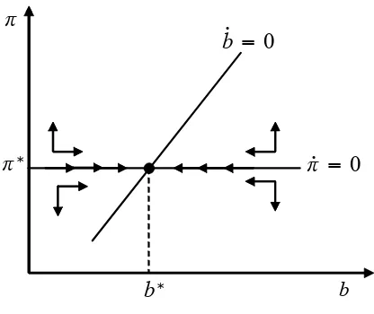
[image:10.595.194.402.128.303.2]b
Figure 1: Passivefiscal policy and active monetary policy
whereA21 = (b∗ +K∗) (φ0−1)−m∗
³
1−η∗m/π´, withη∗m/π =|(π∗/m∗)m0φ0|
denoting the elasticity of money demand with respect to inflation, evaluated at (π∗, b∗).
Since bis a state variable and π a jump variable, we have a saddle path if the following condition holds:
detJ =H∗(φ0−1) (ρ−α)<0. (18)
Condition (18) is satisfiedeither if «α > ρandφ0 >1» (passivefiscal policy
and active monetary policy) or if «α < ρ and φ0 <1» (active fiscal policy
and passive monetary policy). These are the two cases that specify Leeper’s dichotomy. To see it at work, suppose to start from a value b0 6=b∗.
Whenα > ρ, the solution of the system (16) is given by
½
b=b∗+ (b0−b∗)e−(α−ρ)t,
π=π∗. (19)
Since, by assumption, fiscal policy is passive, the monetary authority is per-fectly able to control inflation according to the Taylor principle (φ0 > 1).
The phase diagram of the system (16) is presented in Figure 1. The slope of the locusb˙ = 0, given by(ρ−α)/A21, depends on the sign of A21 which can
the government, since, by assumption,φ0 >1; on the other hand, it increases
inflation tax. In Figure 1, we have drawn the locusb˙ = 0with positive slope, as it is more likely to occur when inflation is relatively low. Nevertheless, this slope has no relevance for the system dynamics, since in this case the saddle path coincides with the locus π˙ = 0. Finally, equation (19) implies that the velocity through which debt converges to the steady state is an increasing function of α.
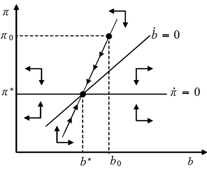
Whenα < ρ, we must haveφ0 <1for saddle-path stability to occur. The
solution of the system (16) becomes
½
b=b∗+ (b0−b∗)eH
∗(φ0−1)t
,
π =π∗+S(φ0, α) (b−b∗). (20)
where S(φ0, α) = −TrJ/A
21 > 0 measures the slope of the saddle path,
which is greater than the slope of the locus b˙ = 0. Since nowfiscal policy is active (α < ρ), the monetary authority cannot follow the Taylor principle. Assuming b0 > b∗, the jump in inflation above the target π∗ allows the real
public debt to decrease gradually and converge to the steady state. This is because
∂b˙ ∂π
¯ ¯ ¯ ¯ ¯
(π∗,b∗)
=A21 <0. (21)
The intuition is as follows. Inflation decreases the real interest rateφ(π)−π, increases inflation tax, and hence increases the monetaryfinancing of deficit.4
The associated phase diagram is illustrated in Figure 2. The jump in inflation needed to ensure stability of real public debt is in accordance with the so-called “fiscal theory of the price level”.5 In synthesis, when fiscal policy is
active, inflation dynamics depends on fiscal variables.
To summarize, Leeper’s dichotomy establishes that monetary policy is able to control inflation consistently with the target level π∗, provided that
fiscal policy takes the burden of controlling public debt. In the opposite case, it is monetary policy that must take the burden of bringing public debt back to the level b∗. Monetary policy can obtain this result only by allowing
inflation to jump above the levelπ∗ when b(t)> b∗.
4The termA
21 can be decomposed in two parts. The first part is negative only when
φ0 <1. The second part is negative if the economy is on the upward-sloping side of the Laffer curve for seignorage, as it is efficient.
b
0
b 0
b b0
[image:12.595.194.402.127.303.2]0
Figure 2: Active fiscal policy and passive monetary policy
Thus, Leeper’s dichotomy states that a necessary condition for monetary policyindependence in the presence of public debt is thatfiscal policy is pas-sive. In the next Sections, we explore the constraints that thefiscal authority can face in implementing a passive policy, as soon as we relax the simplified case of lump-sum taxation.
3
Bonds taxation and the participation
constraint
We have seen that fiscal policy is passive when its primary objective is pub-lic debt stabilization. To obtain this result, the implicit marginal tax rateα
must be greater than ρ, the steady-state real return on public bonds. This condition raises a feasibility problem for a passivefiscal policy, which emerges when we remove the assumption of lump-sum taxation, thus enabling opti-mizing households to take into account the interaction between their choices and the level of taxation.6 Intuitively, the household will never demand an
asset with a negative real return.7
6As long as taxation is lump sum and equilibrium is competitive, so that the single household is atomistic, the exogenous parameterαdoes not appear in the solution of the private agents’ maximizing problem. This is because the representative household is not able to internalize taxation into its optimal choice.
Let us analyze the argument. Suppose that fiscal policy obtains its rev-enues by setting the nominal public debt as tax base,8 with a tax rate equal
to α. The households’ participation constraint in the bonds market imposes
α < i. (22)
We shall now show that, by rewriting the model with such a participation constraint, fiscal policy cannot be passive.
The representative household’s instant budget constraint in real terms is now
c+b˙+m˙ = (i−π−α)b+y−α¯+τh−πm. (23)
Performing optimization yields
(1) uc(c, m) =λ,
(2) um(c, m) =λ(i−α),
(3) λ˙ =λ(ρ+π+α−i).
(24)
The government’s budget constraint is now
g+τh+ (i−π−α)b−α¯−πm=b˙+m.˙ (25)
In equilibrium, optimality conditions (24.1) and (24.2) can be written in implicit form as follows:
½
(1) m=m(i−α) with m0 <0,
(2) λ=λ(i−α) with λ0 <0. (26)
The closed-form differential-equation system in the variables (π, b) is then given by
˙
π=H(π) [φ(π)−π−α−ρ], (27)
˙
b= [φ(π)−π−α]b+g+τh+K(π) [φ(π)−π−α−ρ]−πm[φ(π)]. (28)
The steady-state solutions are
φ(π∗) =α+ρ+π∗, (29)
b∗ = α¯−g−τh+π∗m(α+ρ+π∗)
ρ . (30)
It immediately follows that
∂b˙ ∂b
¯ ¯ ¯ ¯ ¯
(π∗,b∗)
=ρ. (31)
This proves that fiscal policy cannot be passive, for households internalize bonds taxation into their optimal decisions.
The implications for monetary policy are straightforward. Now, the Ja-cobian is
J =
·
H∗(φ0−1) 0
A21 ρ
¸
. (32)
The emergence of a saddle path requires φ0 <1, that is, a passive monetary
policy. The monetary authority is no longer able to control inflation.
To conclude, a passive fiscal policy cannot rely on debt taxation only. There are two alternatives to ensure macroeconomic stability. Thefirst is to combine debt taxation with an inflationary path brought about by a passive monetary policy, along the lines depicted by the fiscal theory of the price level. But in this case, the monetary authority cannot be independent, i.e., cannot adopt a Taylor-type rule withφ0 >1, in order to set inflation equal to
the target level π∗. The second alternative is to raise revenues from another
tax base.
4
Income taxation in an endowment economy
Let us focus on the implications of using income taxes as instrument of a passive fiscal policy.9 For now, let us maintain the simplified hypothesis of
endowment economy. So the analysis of this Section is directly comparable with Leeper’s (1991), and serves to introduce the issues addressed in the next Section.
Letτy <1be the tax rate on income. The household’s budget constraint
is given by
c+b˙+m˙ = (i−π)b+ (1−τy)y+τh−πm. (33)
Since y is exogenous, the optimality conditions are exactly the same as in Section 2.
The government’s budget constraint is given by
g+τh+ (i−π)b−τyy−πm=b˙+m.˙ (34)
Fiscal policy is now described in terms of a feedback rule in which income taxation reacts to public debt:
τyy= ¯α+αb. (35)
The differential-equation system is the same as in Section 2. Hence, using income, as opposed of debt, as tax base allows to reestablish Leeper’s di-chotomy, so that a passivefiscal policy allows monetary policy independence. However, this result is subject to the following remark.
The steady-state marginal tax rate, τ∗y, depends on the target inflation rateπ∗, independently set by the monetary authority, and on the steady-state level of public debt b∗:
τ∗y =ρb
∗
y +
g+τh
y −
π∗m(ρ+π∗)
y . (36)
From (36), the fiscal rule may violate the participation constraint, which imposes τy < 1. Because ∂τ∗y/∂b∗ > 0, it emerges a limit on the level
of steady-state public debt. Let bM
y be the threshold value of public debt
beyond which the participation constraint is violated. From (36), it follows that
bM
y =
y−g−τh+π∗m(ρ+π∗)
ρ . (37)
Ifb0 > bMy , it is not feasible to implement a passivefiscal policy, forτy(0)y =
¯
α+αb0 >1, which violates the constraint τy <1. A central bank intended
to follow the Taylor principle has to accept a higher steady-state inflation rate in order to raise the monetary financing, thereby ensuring b0 ≤bMy .
The foregoing remark, it can be argued, is “purely” theoretical. The condition b0 > bMy could be, in fact, empirically implausible. However, recall
optimal decisions andfiscal revenues no longer holds in a production economy. We shall examine the consequences in what follows.
5
La
ff
er e
ff
ects and monetary policy
independence
Consider an economy populated by a continuum of identical household-firms. The production technology of the representative household-firm is given by
y=l, (38)
where l represents labor supply. The household’s lifetime utility function takes the following form:
U =
∞
Z
0
e−ρt[u(c, m) +f(g)−v(l)]dt, (39)
where u(c, m)is linearly homogeneous, so that uccumm−u2cm = 0, v0(l)>0
andv00(l)>0.
Using (38), the household-firm’s flow budget constraint is given by (33), and the optimality conditions associated with the maximization problem
be-come
(1) uc(c, m) =λ,
(2) um(c, m) =λi,
(3) v0(y) =λ(1−τ
y),
(4) λ˙ =λ(ρ+π−i).
(40)
The government’s budget constraint is given by (34). Fiscal policy is described by rule (35).
In equilibrium, conditions (40.1)-(40.3) can be expressed in implicit form as10
(1) y=y(i, τy) with yi <0, yτy <0,
(2) m=m(i, τy) with mi <0, mτy <0,
(3) λ=λ(i) with λ0 <0.
(41)
Using (41.1), the fiscal policy rule takes the following form:
τyy(i, τy) = ¯α+αb. (42)
Differentiating with respect to time yields
˙
τy =
α
y³1−ηy/τy´
˙
b− τyyi y³1−ηy/τy´
˙
i, (43)
whereηy/τy =¯¯(τy/y)yτy
¯
¯denotes the elasticity of output with respect to the marginal rate. We assumeηy/τy <1, i.e., that the economy is on the upward-sloping side of the Laffer curve, for it results to be efficient. Therefore, we can write
τy =τ(b, i) with τb >0, τi >0. (44)
Dynamics can then be expressed in terms of the following differential-equation system:
˙
π =H(π) [φ(π)−π−ρ], (45)
˙
b=[φ(π)−π−α]b+g+τh−α¯+K(π, b)[φ(π)−π−ρ]−πm{φ(π), τ[b, φ(π)]} 1 +mτyτb
,
(46) where K(π, b) =λ¡mi+mτyτi
¢
/λ0 >0.
The steady-state solutions are given by
φ(π∗) =ρ+π∗, (47)
b∗ = α¯−g−τh+π∗m[ρ+π∗, τ(b∗, ρ+π∗)]
ρ−α . (48)
It follows that
∂b˙ ∂b ¯ ¯ ¯ ¯ ¯
(π∗,b∗)
= ρ−α−π∗mτyτb
= ρ−α
1 + π
∗m τy
y∗³1−η∗ y/τy
´
, (49)
where we have used the fact that, from (44) evaluated at the steady state,
τb =α/y∗ ³
1−η∗ y/τ
´
To facilitate our discussion on dynamic stability, and make the present analysis easily comparable with the results that apply in the benchmark model of Section 2, let us restrict attention to the case in which
y∗³1−η∗y/τy
´
>¯¯π∗mτy
¯
¯. (50)
This condition simply says that the increase in fiscal revenues generated by an increase in the tax rate is greater than the decrease in inflation tax brought about by the associated fall in money demand. Therefore,total revenues, i.e.,
fiscal revenues plus inflation tax, are assumed to raise following an increase in the tax rate. If condition (50) holds, then a passivefiscal policy requires
α > ρ
1 +π∗m τy/y∗
³
1−η∗ y/τy
´. (51)
Since π∗mτy/y∗
³
1−η∗y/τy´<0, the feedback parameter α must be greater than in the endowment-economy case. The reason is clear. An increase in public debt causes the tax rate to raise via the fiscal policy feedback rule. The increase in the tax rate brings about a decrease in output and hence in money demand. This crowds out inflation tax, thereby requiring a more aggressive reaction by the fiscal authority. The foregoing mechanism implies that the higher the elasticity of output with respect to the tax rate, the higher parameter α ensuring a passive fiscal policy, as it is apparent from (51).
The Jacobian is given by
J =
H
∗(φ0−1) 0
B21 ρ−α
·
1 + π∗mτ y y∗1−η∗
y/τ y
¸
, (52)
where
B21=
(b∗+K∗) (φ0−1)−m∗³1−η∗ m/π
´
−π∗mτyτiφ
0
1 +mτyτb
for saddle-path stability. The latter occurs if the following condition applies:
detJ =H∗(φ0 −1)−ρ−α
1 + π
∗m τy
y∗³1−η∗ y/τy
´
<0. (53)
Condition (53) is verified either if
α > ρ
1 +π∗mτ
y/y∗
³
1−η∗ y/τy
´ and φ0 >1
or if
α < ρ
1 +π∗mτ
y/y∗
³
1−η∗ y/τy
´ and φ0 <1.
If fiscal policy is passive, i.e., α > ρ/h1 +π∗m τy/y∗
³
1−η∗ y/τy
´i
, monetary policy independence is ensured.
However, for a given target inflation rate independently set by the mone-tary authority, the occurrence of Laffer-type effects poses a limit on the level of steady-state public debt. Let indicate it bybM
l . We shall demonstrate that
beyond such a limit, a passive fiscal policy becomes unfeasible.
To prove this result, first notice that in the steady state it must be that
τ∗yy¡ρ+π∗, τ∗y¢+π∗m¡ρ+π∗, τ∗y¢=ρb∗+g+τh. (54)
It follows that
bMl = max
τ∗y
£
τ∗yy¡ρ+π∗, τ∗y¢+π∗m¡ρ+π∗, τ∗y¢¤−g−τh
ρ . (55)
Maximization of total revenues with respect to the tax rate occurs when
y∗³1−η∗y/τy´=−π∗mτy. (56)
Since mτy < 0, total revenues are maximized on the left-hand-side of the
Now, substituting (56) into (49) yields
∂b˙ ∂b
¯ ¯ ¯ ¯ ¯(π∗,bM
l )
=ρ. (57)
This demonstrates our finding: if b0 > bMl , fiscal policy cannot be passive,
for total revenues cannot be sufficient to reduce public debt over time. Remarkably, the presence of Laffer effects on tax revenues causes the threshold level of public debt to be lower with respect to the endowment-economy case. That is, we have
bMl < bMy . (58)
A central policy implication emerges. If b0 > bMl , the dynamics of public
debt can be controlled only by means of inflation tax revenues. Monetary policy independence is no longer possible.
6
Maximum debt, in
fl
ation targeting, and the
fi
scal theory of the price level
From (55), bM
l is a function of the target inflation rate π∗, blM=bMl (π∗). To
study this function, we can apply the envelop theorem. We have
dbM
l
dπ∗ =
τMy
i+m∗+π∗mi
ρ (59)
= m∗
ρ
µ
1−η∗m/π− τ
My∗
π∗m∗η ∗ y/π
¶
,
where
τM = arg max
τ∗y
£
τ∗yy¡ρ+π∗, τ∗y¢+π∗m¡ρ+π∗, τ∗y¢¤.
From (59), dbM
l /dπ∗ > 0 as long as η∗m/π − ¡
τMy∗/π∗m∗¢η∗
y/π < 1. We let
πMbe the value of the inflation rate such thatη∗
m/π−
¡
τMy∗/π∗m∗¢η∗
y/π = 1,
that is, dbM
l /dπ∗ = 0.
FunctionbM
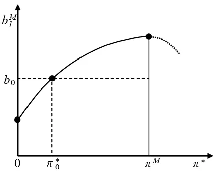
l (π∗)is illustrated in Figure 3, and has the following
interpre-tation. For π∗ = 0, we have η∗
m/π =η∗y/π = 0, so that dblM/dπ∗ =m∗/ρ > 0.
As long asπ∗ raises, both elasticitiesη∗
b0
M
0 0
[image:21.595.193.405.125.299.2]blM
Figure 3: Maximum debt and inflation target
the increase in inflation causes the nominal interest rate to raise, leading to a fall in both money demand and output. As a result, total revenues, that is, fiscal revenues plus inflation tax, increase as long as π∗ < πM, reach a maximum at π∗ =πM, and decrease as along as π∗ > πM. Two implications
for the design of monetary policy rules arise.
First, if the monetary authority is intended to adopt the Taylor principle in order to maintain inflation control around the steady state, and at the same time avoid explosive paths in public debt, itmust set an inflation target such that π∗0 ≤π∗ ≤πM, thereby ensuringb0 ≤bMl .
Second, if the monetary authority sets a target inflation rate such that
π∗ < π∗
0, then we have b0 > bMl , and macroeconomic stability is guaranteed only by inflation dynamics along the lines of the fiscal theory of the price level. In fact, the Jacobian evaluated at ¡π∗, bM
l ¢
is given by
J(π∗,bM
l ) =
·
H∗(φ0 −1) 0
B21 ρ
¸
. (60)
Saddle-path stability requires that monetary policy is passive,φ0 <1.
Violat-ing the Taylor principle allows the inflation rate to jump up in order to rule out explosive dynamics in public debt. Nevertheless, in this second case the monetary authority clearly looses inflation control around the steady state.11
7
Conclusions
Distortionary taxation has negative consequences for monetary policy inde-pendence. It is well known, at least since the original contribution by Leeper (1991), that inflation control by an independent monetary authority requires a passive fiscal policy, ensuring stability of public debt for each time path of inflation. In this paper, we have demonstrated that when only distortionary revenue sources are available for the government, passive fiscal policies may not be feasible. This result comes about because of both households’ partic-ipation constraints and Laffer-type effects. We have shown that there exists a threshold level of public debt beyond which monetary policy independence vanishes. We have examined the implications for policy design. The central bank can maintain inflation control around the steady state, by applying the Taylor principle, provided it targets a higher inflation rate. Otherwise, infl a-tion must endogenously jump up in line with the fiscal theory of the price level.
Appendix A
Consider the two optimality conditions (4.1) and (4.2). Differentiating with
respect to time, recalling that c˙ = 0, we can write the results in matrix notation: µ
ucm −1
umm −i ¶ µ ˙ m ˙ λ ¶ =λ µ 0 ˙ i ¶ . (A.1)
Let ∆=umm−ucmi <0. Then we have
˙ m= λ ¯ ¯ ¯ ¯
0 −1 ˙
i −i
¯ ¯ ¯ ¯ ∆ = λ
∆˙i, (A.2)
˙ λ= λ ¯ ¯ ¯ ¯
ucm 0
umm i˙ ¯ ¯ ¯ ¯ ∆ = λucm
∆ i.˙ (A.3)
We can thus write (10).
Appendix B
Consider the three optimality conditions (4.1)-(4.2). Differentiating with re-spect to time and imposing the goods’ market equilibrium condition, we can express the results as
ucc ucm −1
ucm umm −i
v00 0 −(1−τ
y) ˙ y ˙ m ˙ λ =λ
0 ˙
i
−τ˙y
. (B.1)
Let Ψ=v00(u
mm−ucmi)<0. Hence, we have
˙ y = λ ¯ ¯ ¯ ¯ ¯ ¯
0 ucm −1
˙
i umm −i
−τ˙y 0 −(1−τy) ¯ ¯ ¯ ¯ ¯ ¯ Ψ (B.2)
= λ(1−τy)ucm
Ψ ˙i−
˙
m =
λ
¯ ¯ ¯ ¯ ¯ ¯
ucc 0 −1
ucm i˙ −i
v00 −τ˙
y −(1−τy) ¯ ¯ ¯ ¯ ¯ ¯
Ψ (B.3)
= λ[v
00−(1−τ
y)ucc]
Ψ i˙+
λ(ucm−ucci)
Ψ τ˙y,
˙
λ =
λ
¯ ¯ ¯ ¯ ¯ ¯
ucc ucm 0
ucm umm ˙i
v00 0 −τ˙
y ¯ ¯ ¯ ¯ ¯ ¯
Ψ (B.4)
= λv00ucm
Ψ i.˙
References
Bénassy, J. P. (2007), Money, Interest and Policy: Dynamic General Equi-librium in a non-Ricardian World, MIT Press, Cambridge MA.
Cochrane, J. (1998), “A Frictionless Model of U.S. Inflation”, in Bernanke B. S. and J. J. Rotemberg, eds.,NBER Macroeconomics Annual 1998, MIT Press, Cambridge MA, 323-384.
Cochrane, J. (2005), “Money as Stock”,Journal of Monetary Economics 52, 501-528.
Edge, R. M. and J. B. Rudd (2007), “Taxation and the Taylor Principle”,
Journal of Monetary Economics 54, 2554-2567.
Leeper, E. M. (1991), “Equilibria under ‘Active’ and ‘Passive’ Monetary and Fiscal Policies”, Journal of Monetary Economics 27, 129-147.
Leeper, E. M. and T. Yun (2006), Monetary-Fiscal Policy Interactions and the Price Level: Background and Beyond”,International Tax and Pub-lic Finance 13, 373-409.
Linnemann, L. (2006), “Interest Rate Policy, Debt, and Indeterminacy with Distortionary Taxation”, Journal of Economic Dynamics and Control
30, 487-510.
Schmitt-Grohé S. and M. Uribe (2007), “Optimal Simple and Implementable Monetary and Fiscal Rules”,Journal of Monetary Economics54, 1702— 1725.
Sims, C. (1994), “A Simple Model for Study of the Determination of the Price Level and the Interactions of Monetary and Fiscal Policy”, Economic Theory 4, 381-399.
Taylor, J. B. (1993), “Discretion Versus Policy Rules in Practice”, Carnegie-Rochester Conference Series on Public Policy 39, 195-214.
Woodford, M. (1995), “Price-Level Determinacy without Control of a Mone-tary Aggregate”,Carnegie-Rochester Conference Series on Public Pol-icy 53, 1-46.