Is the US Demand for Money Unstable?

Munich Personal RePEc Archive

Is the US Demand for Money Unstable?

Rao, B. Bhaskara and Kumar, Saten

University of Western Sydney, Auckland University of Technology

14 June 2009

Online at

https://mpra.ub.uni-muenchen.de/15715/

Is the US Demand for Money Unstable?

B. Bhaskara Rao

raob123@bigpond.com

University of Western Sydney, Sydney (Australia)

Saten Kumar

kumar_saten@yahoo.com

Auckland University of Technology (New Zealand)

Abstract

The demand for money (M1) for the USA is estimated with annual data from 1960-2008 and its

stability is analyzed with the extended Gregory and Hansen (1996b) test. In addition to

estimating the canonical specification, alternative specifications are estimated which include a

trend and additional variables to proxy the cost of holding money. Results with our extended

specification showed that there has been a structural change in 1998 and the constraint that

income elasticity is unity could not be rejected by subsample estimates. Short run dynamic

adjustment equations are estimated with the lagged residuals from the fully modified OLS

(FMOLS)estimates of cointegrating equation and also with the general to specific approach (GETS).

Keywords: Demand for M1, USA, Structural Breaks, Income Elasticity, Cost of Holding Money

1.Introduction

The US demand for money function and its stability have been analyzed by many studies.

Some often cited works are Goldfeld (1976), Judd and Scadding (1982), Lucas (1988), Poole

(1988), Baba et al. (1992), McNown and Wallace (1992), Stock and Watson (1993), Hoffman et

al. (1995) and Yossifov (1998), Ball (2001) and Choi and Jung (2009).1 Duca and VanHoose

(2004) have surveyed important developments in monetary economics including the need to

study the demand for money and the current view that this relationship is unimportant because

many central banks have abandoned targeting monetary aggregates and switched to the rate of

interest as the monetary policy instrument. However, according to Duca and VanHoose, studying

this relationship is not an irrelevant activity and therefore summarized the salient features of

some key empirical works. Others who take a similar view on the need to study the demand for

money areLeeper and Roush (2003) and Ireland (2004). Ireland has estimated a business cycle

model for the USA within the ISLM model framework augmented with a Phillips curveand with

the post 1980 quarterly data. However, he found that money played relatively a smaller role in

explaining the dynamics of inflation and output. In our view this does not mean that demand for

money is redundant because Ireland’s results are also consistent with instability in the demand

for money which might have contributed to the poor correlation between money, inflation and

output.2 The dependent variable in the demand for money varied from the narrow definition of

money (M1) to broader measure with weighted averages of monetary aggregates. Although some

influential studies have found that the US demand for money (mainly M1) is stable for a long

period up to the early or mid 1970s, others have found that it has become unstable since then due

to financial reforms, improvements in payments technology and cash management practices,

1 _{Studies by Lucas (1988), Poole (1988), Stock and Watson (1993) and Hoffman et al. (1995) asserts that the}

demand for M1 in US is stable over the 20th century. However, Goldfeld (1976) and Judd and Scadding (1982) found that the money demand is unstable during 1970s. Further, McNown and Wallace (1992) and Yossifov (1998) obtained implausible income elasticity of M1 and M2. See Sriram (1999) for a survey.

2 _{The pros and cons on whether monetary aggregates or the interest rate should be used as monetary policy}

which have been significantly improved with parallel progress in computer technology. In this

paper we shall examine if these efficiency effects can be captured with modified specifications to

improve the stability of this relationship and if the income elasticity of the demand for money is

unity as found in many earlier studies. For this purpose, we shall use annual data from 1960 to

2008 for M1.

This paper is organized as follows. Section 2 reviews a few recent contributions on the US

demand for M1. Section 3 discusses our modifications to its canonical specification and presents

estimates of cointegrating equations. Structural break tests are also conducted in this section.

Since these tests have weak power against the null of no cointegration it is necessary to use

discretion to specify and estimate stable demand for money functions. Section 4 concludes.

2. Recent Studies of US Demand for Money

Several pre 1980s studies have generally used annual data and the following canonical

specification for the demand for real money.

0

lnm_t = +θ θ_yln( )y_t +θ_RR_t+ε_t (1)

where θ₀ =intercept, m=real money stock, y=real output, R=cost of holding money proxied

with the nominal short term interest rate and ε ∼N(0, ).σ They found that this function is stable

and estimates of the income elasticity (θy)are about unity and the semi-interest rate

elasticity (θR)is around -0.1. According to Friedman and Kuttner (1992), the above canonical

specification for M1 is cointegrated with income and the rate of interest for the period 1960–

1979, but becomes unstable if samples are extended to include data from the 1980s. However,

Ball (2001), in an insightful study, noted that stability tests did not show breaks in the demand

for M1 with data up to 1987, but a break is generally found if the samples include data through

1996; Duca and VanHoose (2004, p. 259). He also found that when the data are extended beyond

1987, the pre 1970s estimates of income and interest rate elasticities reduce by half so that

0.5 y

More formal break tests are conducted on the US demand for money by Gregory and

Hansen (1996a) with annual (1901-1985) and quarterly (1960Q1-1994Q4) data. They have used

the canonical specification mainly to illustrate their method for testing for a single endogenous

break in a cointegrating equation, and not to examine the adequacy of alternative specifications

of the demand for money. More recently Choi and Jung (2009) have applied the Bai and Perron

(2003) tests for testing for multiple endogenous breaks in the US demand for money. Unlike the

Gregory and Hansen one step tests for cointegration with one break, the Bai and Perron tests are

tests for multiple breaks in equations estimated with OLS. Therefore, it is necessary to test for

cointegration for each subsample implied by these first stage break tests. Choi and Jung have

used a pragmatic option to test for multiple breaks because there is no formal test so far to test

for cointegration with multiple endogenous breaks in a single step. Furthermore, the main

objective of Choi and Jung seems to be to illustrate the use of the Bai and Perron tests for testing

for multiple endogenous breaks with the canonical specification of the demand for money and

not to examine the merits of alternative specifications of this relationship.

Gregory and Hansen found an intercept break in 1941 in their annual data, but in their

quarterly data there is only weak evidence for both an intercept and slope shift in 1975Q2. In

contrast Choi and Jung, using quarterly data (1960Q1 to 2000Q2), have found that there are two

breaks in the US demand for money in 1974Q2 and 1986Q1. Therefore they tested for

cointegration with the Johansen maximum likelihood method (JML) and found one cointegrating

equation for each of the 3 subsamples implied by their break tests. However, instead of reporting

JML estimates of the cointegrating equations, which should have been straightforward, they

reported estimates with the 4 alternative methods.3 Since we shall use later the Phillips and

Hansen fully modified OLS method (FMOLS) to estimate the cointegrating equations, besides

JML, we shall briefly summarize Choi and Jung’s findings based on FMOLS. They found that in

the first subsample (1959Q1–1974Q1) income elasticity was 0.33 and increased to 0.49 in the

second subsample (1974Q2–1986Q1) and then declined to 0.25 in the third subsample (1986Q2–

3

2000Q2).4 Estimates of semi-interest rate elasticity was insignificant in the first subsample but

increased in absolute value to -0.045 and became significant in the third subsample. They did not

report estimates of the intercepts.

These aforesaid works provided valuable insights and in particular Choi and Jung are the

first to test formally for structural breaks in the demand for money function of the USA.5

However, a weakness in the previous studies is that there is no trend in their specifications. In

fact many other earlier studies have also ignored trend including a path breaking work by Baba et

al. (1992). Ideally the following specification with trend could be estimated to capture some

effects of improvements in the transactions technology.6

0

lnmt = +θ θTTrend+θylnyt+θRRt+εt (2)

There is a problem with including trend. As Ball has pointed including trend may give

unreliable estimates of the parameters because of the high colinearity between trend and income.

Therefore, he has also estimated cointegrating equations with the constraint that income

elasticity is unity and these estimates turned out to be informative and did not change his major

finding that the demand for money has become unstable when the sample size is extended

beyond the late 1980s and up to the mid 1990s.

The specification in (2) may be still inadequate because it can be extended to include other

variables that could better proxy the cost of holding money. For example, in addition to the short

term interest rate, the inflation rate and exchange rate can be used by money holders to proxy the

cost of holding money because inflation reduces the real value of money. As Choi and Jung have

noted, it is likely that cash management practices might have significantly changed after the

introduction of the flexible exchange rates in 1973. Ignoring these variables in the demand for

money may also cause instability in this relationship. However, the usefulness of such extensions

depends on the empirical results, but inclusion of these two additional variables is justified when

4 _{Unfortunately Choi and Jung’s dating the break dates gives the impression that they are using monthly and not}

quarterly data. Therefore, our notation of the dates for the subsamples based on what they might have intended to. 5 _{Gregory and Hansen used the demand for money to illustrate their techniques and per se they are not interested in a}

wider sense in the issues on the demand for money. Rao and Kumar (2007, 2009) have used their tests for testing structural breaks in the demand for money of Fiji and Bangladesh.

the Fisher condition holds only weakly i.e., the correlation between the rate of interest and

inflation is not high. In our sample this correlation is about 0.6 and the correlation between the

rate of interest and REER is very low.7 Subject to this caveat our extended specification of the

demand for money is:

0

ln ln( )

ln ln( ) (3)

t T y t R t

p t x t t

m Trend y R

P REER

θ θ θ θ

θ θ ε

= + + +

+ ∆ + +

where ln( )∆ P =rate of inflation and REER=real effective exchange rate. This improved

specification may improve the stability of the demand for money and or show that the structural

changes are minor.8 We shall estimate (3) in the following section. Definitions of the variables and data sources are in the appendix.

3. Empirical Results

In this section we shall estimate the cointegrating equations for the demand for money

(M1) with alternative specifications and sample periods with annual data from 1960 to 2008. The

Phillips and Hansen FMOLS method is used because it is simpler and quick to implement and

convenient to estimate a number of cointegrating equations with different specifications and

sample periods. However, there is no formal cointegration test for FMOLS estimates and the

significance of the coefficients is generally used for the validity of the estimated cointegrating

equations. Therefore, we shall use, on a selected basis, the Johansen maximum likelihood (JML)

test for cointegration, as in Choi and Jung, and report estimates of the JML cointegrating

equations if they are plausible. Finally, we shall estimate the short run dynamic adjustment

equations with the lagged residuals from the FMOLS equations and also with the general to

7 _{See Baba et al. (1992, p.29) for a similar reasoning for the inclusion of the rate of inflation. In our sample the}

correlation between interest rate and inflation rate is about 0.7 implying that 49% of interest changes are explained by inflation.

8 _{Baba et al. analyzed the US demand for money from this perspective and although they did not conduct formally}

specific approach (GETS) of the London School of Economics, of which David Hendry is the

most ardent exponent.

In Table 1 the estimated cointegrating equations with FMOLS for specifications in (1) to (3) are

reported in the first 3 rows. All the estimated coefficients are significant at the 5% level but

estimates of income elasticities change significantly with the specifications. While the estimate

of income elasticity (θy) is the low at about 0.2 in the canonical specification, it has increased to

about 0.5 when trend is added. Only in our extended specification in equation (3) θy =1.0178

and equal to its stylized value of unity.

The cointegrating equations with JML are estimated for equations (3) and (1) and reported,

respectively, in rows 4 and 5 of Table 1 to highlight the improvements with our extended

specification. Both the trace and maximal eigenvalue tests could not reject the null of a single

cointegrating equation.9 The estimated income and interest rate elasticities in the extended

equation (3) are close in both the FMOLS and JML estimates with some differences in the

coefficients of inflation and real effective exchange rate. JML estimates of these two parameters are more in absolute magnitude than in FMOLS. There are significant differences in the FMOLS

9 _{To conserve space we report below only the Maximal Eigenvalue test for (3) and (1).}

H0 H1

Equation (1)

Test Statistic 95% CV

Equation (3)

Test Statistic 95% CV

r = 0 r = 1 49.377 37.860 81.231 22.040

r<= 1 r = 2 30.884 31.790 5.963 15.870

r<=2 r = 3 13.189 25.420 3.754 9.160

Table 1 Estimates of Cointegrating Equations

Method Period Equation θ₀ θ_T θ_y θ_R θ_p θ_x

FMOLS 1962-2008 EQ 1 1.412

(9.89)*

0.185

(11.60)*

-0.009

(3.51)*

FMOLS 1962-2008 EQ 2 -1.033

(0.53) -0.010 (1.28) 0.496 (2.00)* -0.011 (4.24)*

FMOLS 1962-2008 EQ 3 -3.900

(3.05)* -0.035 (6.31)* 1.018 (6.19)* -0.013 (5.52)* -1.177 (4.29)* -0.431 (5.57)*

JML 1962-2008 EQ 3 @ -0.033

(2.88)* 0.928 (2.83)* -0.014 (3.42)* -2.282 (4.02)* -0.347 (3.31)*

JML 1962-2008 EQ 1 4.457

(0.97)

-0.071

(0.18)

-0.058

(0.78)

Notes: @ = Estimated with unrestricted intercepts and restricted trends in the VAR. C = Constrained equation. Absolute t-ratios are in the parenthesis. Significance at 5% level is represented by *.

and JML estimates of the canonical specification in (1). Estimates of income and interest rate

elasticities are lower but significant in FMOLS, but neither is significant in the JML estimates.

Since our extended specification seems to be more robust, we select this to test for structural

breaks. The estimate of the trend coefficient of this equation implies that demand for money has

been declining at the rate of about 3.5% per year due to financial reforms and improvements in

payments technology. However, as noted by Ball, the estimate of the coefficients of trend and

income are unlikely to be accurate due to the high colinearity between these two variables. We

shall discuss this problem later.

We shall use the Gregory and Hansen (1996b) extended break test to test for cointegration

with a single structural break with the trend variable in the specification. When this test is

implemented we found that there is no cointegration with a significant break in the extended

equation (3). The test results are in row 1 of Table 2. This result may partly be due to colinearity

that θ_y =1 in (3). This is a reasonable assumption because in both the FMOLS and JML

estimates, the constraint thatθ_y =1could not be rejected at the 5% level by the Wald test. Test

results, in row 2 of Table 2, with this modification also failed to detect a significant break.

However, the identified break date is 1998 but it should be noted that this is not significant even

at the 10% level. To increase the degrees of freedom and efficiency of the test, we have proxied

the cost of holding money with the principal component (PC) of ,R ∆DLPand LREER and the

specification with this modifications is as follows.

lnm_t−lny_t =Intercept+θ_TTrend+θ_pcPC_t (4)

where the dependent variable can also be interpreted as the inverse of velocity. When (4) is

tested for a break, the test statistic (absolute value) is only marginally less than the CV (absolute

value) at the 10% level, also indicating a break in 1998 and the results are in row 3 of Table 2.

These break test results should be taken with some caution for a few reasons. Firstly, the

Gregory and Hansen tests are joint tests for cointegration with a structural break and there may

actually be cointegration without a structural break. Secondly, there may be more than one break

and both the intercept and slope coefficients may change. Thirdly, they have low power against

the null of no cointegration and discretion is necessary to interpret them.

Table 2 Tests for Cointegration with a Structural Break

Specification Test statistic

5% CV 10% CV Break Date

1 _{ln ln( )}

ln ln( )

T y t

p t x t

t

m Intercept Trend y

P REER

θ θ

θ θ

= + + +

+ ∆ +

-6.20 -6.84 -6.58 1990

2 ln ln

ln ln( )

T R t p t x t

t t

m y Intercept Trend R P REER

θ θ

θ θ

= + +

+ ∆ +

− -5.64 -6.32 -6.16 1998

3 _ln

ln _T

pc t

t t

m Intercept Trend

PC

y θ

θ

= +

+

With a somewhat weak but not a totally unsatisfactory test result for a structural break, we

proceeded further as follows. We have estimated the cointegrating equations for the subsamples

(implied by a break in 1998) for the specification in (4) in both an unconstrained and constrained

form on θ_y. The dependent variable in the former is lnm and in the latter (lnm−ln )y and these

formulations help also to test if the income elasticity is unity in both subsamples viz., 1962-1997

and 1998-2008. Both FMOLS and JML methods are used for estimating the cointegrating

equations but JML did not yield any meaningful results for the second subsample perhaps

because there are only 11 observations.10FMOLS estimates are good and given in Table 3. While

estimates in the unconstrained equations that is the intercept, the coefficients of Tand lnyare

almost equal in both subsamples, the coefficient of PC is higher in the second subsample.

However, a Wald test rejected the null that all the coefficients are equal in both subsamples. The

computed test statistic, with p-value in square brackets, is 2 ( 4)

χ =420.845[0.000]. Although point

estimates of income elasticity are about 0.7, a Wald test could not reject the null that income

elasticity in both subsamples is one at the 5% level. The computed test statistics for the first and

second subsamples are 2 (1)

χ =3.143[0.076] and 2 (1)

χ =0.697[0.404]. Next we have re-estimated

with FMOLS the cointegrating equations for both subsamples with the constraint that income elasticity is unity and these are in the third and fourth rows of Table 3.

10 _{Perhaps this may be the reason why Choi and Jung did not report JML estimates of the cointegrating equations for} their subsamples even though JML procedure has been used to test for cointegration. In our JML estimates for the subsample all the estimated coefficients are insignificant but are correctly signed. In the second subsample the coefficients of income and trend are wrongly signed and all are insignificant. Our results imply that perhaps FMOLS

Table 3 Estimates of Cointegrating Equations for Subsamples

Method Period Equation θ₀ θ_T θ_y θ_PC

FMOLS 1962-1997 EQ 4

Unconstrained -2.579 (1.83)** -0.015 (2.72)* 0.684 (3.84)* -0.035 (8.41)*

FMOLS 1998-2007# EQ 4

Unconstrained -2.621 (0.83) -0.014 (1.44) 0.676 (1.74)** -0.043 (5.36)*

FMOLS 1962-1997 EQ 4

Constrained

-5.074

(381.63)*

-0.025

(44.99)*

1.00 -0.036

(7.84)*

FMOLS 1998-2008 EQ 4

Constrained

-5.293

(146.72)*

-0.022

(26.49)*

1.00 -0.053

(8.91)*

Notes: # Inclusion of data for 2008 caused convergence problems and we estimated with data to 2007.

pc

θ =Coefficient of the principal component of R, DLP and LREER. Absolute t-ratios are in the parenthesis. Significance at 5% and 10% levels are denoted by * and **.

Estimates of trend have increased in both subsamples compared to the unconstrained

estimates in rows 1 and 2. Although the coefficients of PC have remained the same in the first

subsample in both the unconstrained and constrained estimates, it has increased in absolute value

in the constrained estimates of the second subsample. A Wald test that all the coefficients in both

subsample equations in rows 3 and 4 are equal has rejected the null. We then tested that each

individual coefficient is the same in both subsamples in rows 3 and 4. The computed 2

χ test

statistics for the null that intercept and the coefficients of trend and PC, with p-values in the

square brackets, are respectively: 270.271 [0.000], 31.309 [0.000] and 13.744 [0.000] indicating

they differ significantly even at the 1% level. Therefore, we may conclude that there has been a

structural change in the US demand for money in 1998 and in particular the intercept and the

response to the cost of holding money have increased in absolute magnitude after 1997.

It would be interesting and informative to proceed further and estimate the short run

dynamic equations based on the cointegrating equations with a structural change. We shall use

the cointegrating equations, based on FMOLS, for the two subsamples in Table 3. Next we shall

use the GETS approach. In contrast to various cointegration methods, where the dynamic short

run equation is estimated in two steps, the dynamic equation with the cointegrating equation can

be estimated in one step with GETS. Recent studies seem to have neglected the short run

dynamic equations of the demand for money and satisfied with estimating the cointegrating

equations and it is not known if estimating long run relationships without short run dynamics

would give robust and reliable estimates of the cointegrating equations.11 In this respect GETS

approach has an advantage over conventional cointegration methods. We have used PcGets to

select the optimal lag structure for the dynamic equations in both methods. The search

procedures in PcGets minimize the path dependent biases; see Hendry and Krolzig (2001) and

Rao and Singh (2006). PcGets has selected, for the whole sample period, a parsimonious lag

structure for the short run equation with the 2 lagged ECM terms, implied by the FMOLS

estimates for the constrained specification in Table 3. The estimate of the parsimonious equation

(5) is as follows.

1 1

1

(4.64)* (2.87)* (6.01)*

(ln ln ) 0.624 97 1.600 08 0.031

0.030 0.797 (l

t t t t t

t

m y ECM ECM PC

PC − − − ∆ − = − − − ∆ ∆ + ∆ 2 ___

2 2 2 2

1 1

(5.59)* (9.41)*

0.494;SER = 0.019

1.664(0.197); 5.328(0.021); 1.785(0.410) ; 0.

n ln )

_{sc ff nn hs}

t t

R

m y

χ χ χ χ

− −

=

= = = =

−

835(0.361) (5)

All the coefficients in (5) are significant at the 5% level and the adjustment coefficients are

correctly signed. The

2 ___

R at about 0.5 is satisfactory and the χ2

tests on the residuals indicate no

serial correlation and non-normality in the residuals. However, the functional form

misspecification test is only insignificant at the 1% level but becomes significant at 2%. It may

be noted that search for a dynamic structure is an empirical issue and it is hard to discover the

11 _{Perhaps the exception is Baba et al. (1992) who estimated with quarterly data (1960Q3-1988Q3) demand for}

correct dynamic structure. The estimate of the adjustment coefficient for the second subsample

period at -1.6 is more than twice for the first subsample of -0.6, implying that the speed of

adjustment towards equilibrium has substantially increased after 1997. Since the absolute value

of the adjustment coefficient for the second subsample exceeds unity, there would be fluctuations

in the adjustment path around the equilibrium value.12 The coefficient of ∆PCtis negative and

its one period lagged value is positive implying that there would be an immediate decrease in the

demand for money when the cost of holding money increases but then this is offset by an

increase in the next period offsetting the previous effect. The coefficient of the lagged dependent

variable is large at 0.8 implying that there is considerable persistence in the changes of the

demand for money. Although the plots of predicted and actual values in Figure 1 and residuals in

Figure 2 seem satisfactory, there are some large positive and negative errors that exceed 2% in

absolute magnitude. There are 17 such errors and 12 are in the first subsample.13

GETS estimate of the demand for money with a dummy variable D98 (zero up to 1997 and 1 afterwards) to allow for a structural change in the cointegrating equation and with the

constraint that income elasticity is unity are in equation (6) below.

1 1 1

(3.52)* (215.36)* (38.56)* (6.24)*

( ln ln ) 0.516(1 98)((ln ln ) ( 5.084 0.025 0.036 ))

t t t t t

m y D m₋ y₋ T PC₋

∆ − ∆ = − − − − − − −

1 1 1

(2.36)* (59.28)* (11.56)* (2.46)*

1.003 98((ln ln ) ( 5.245 0.022 0.038 ))

t t t

D m₋ y₋ T PC₋

− − − − − −

1 1 1

_

(5.28)* (3.03)* (2.56)*

0.031 PC_t 0.020 PC_t 0.408 (lnm_t lny_t )

R

− − −

− ∆ + ∆ + ∆ −

2 2 2 2

2 __

0.519;SER=0.019

0.958(0.328); 11.245(0.001); 0.464(0.793); 0.003(0.982)

sc ff nn hs

χ χ χ χ

=

= = = =

(6)

12 _{Generally it is mistaken that if the adjustment coefficient exceeds unity there is no convergence. However this is}

valid only if the absolute value of the coefficient exceeds 2 but there would be fluctuations in the adjustment path if the estimate is unity or more than unity but below 2.

Figure 1: Plot of Actual and Fitted Values

Plot of Actual and Fitted Values

DLMY

Fitted

Years

-0.02

-0.04

-0.06

-0.08 0.00 0.02 0.04 0.06

19631965 1967 19691971197319751977 1979 198119831985198719891991 1993 19951997199920012003 2005 2007 2008

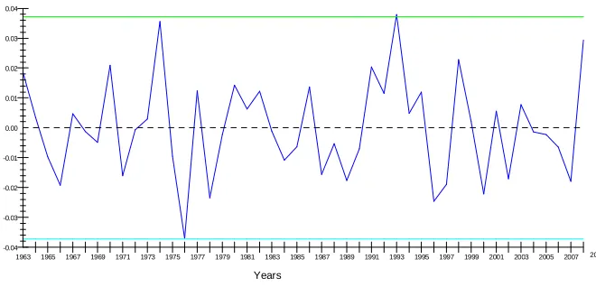
Figure 2: Plot of Residuals and Two Standard Error Bands

Plot of Residuals and Two Standard Error Bands

Years

-0.01

-0.02

-0.03

-0.04 0.00 0.01 0.02 0.03 0.04

All the estimated coefficients are significant in equation (6) at the 5% level and theχ2

tests

on the residuals, except the functional form test as for equation (5), are insignificant. The 2 ___ R at about 0.52 is satisfactory and a trifle more than for equation (5). A Wald joint test with the null

that all the coefficients in both subperiods are equal is rejected at the 5% level. However, Wald

tests on estimates of individual coefficients of the intercepts, adjustment coefficients and the

slopes are equal produced mixed results. While the test did not rejected the null that the

intercepts are equal at the 5% level, this null is rejected at the 10% level. The null that the

adjustment and slope coefficients are equal is not rejected at the 5% level. Since the joint test that

all the combined coefficients are equal has rejected the null, we may conclude that there has been

a structural change in the US demand for money in 1998 and ignore the tests on the equality of

individual coefficients. However, unlike in equation (5), in equation (6) it is possible to test

which coefficients in the cointegrating equation have also changed because in GETS the

parameters in the cointegrating equation and the short run dynamics are estimated in one step.

Based on the point estimates of the individual coefficients, there has been significant

improvement in the speed of adjustment to equilibrium after 1997. While the intercept shifted

down and there is a marginal improvement in the long run response to changes in the cost of

holding money, the change in the coefficient of trend is very small. In the short run dynamics

part of the equation (6) the effect of a changes in the cost of holding money is similar to (5) but

the change in its lagged value has a smaller effect. The coefficient of the lagged dependent

variable is smaller indicating decreased persistence. The plots of the actual and predicted values

are in Figure 3 and the errors in Figure 4. In contrast to equation (5) the number of large errors,

exceeding 2%, in (6) are less. There are only 10 such errors and 7 are in the first subsample. The

years in which the errors exceed 2% are 1970, 1974, 1976, 1978, 1991, 1993, 1996, 1998, 2000,

and 2008. While our GETS estimates could not explain the missing money episode of

1974-1976, the error in 1975 is less than 1%. However, errors in 1974 and 1976 are about 3.5%. Our

equation has adequately explained the great velocity decline of 1982-1983 and M1 explosion of

1985-1986. Errors in these two episodes are less than 1% but the error in 1986 is 1.4% (see Baba

et al. (1992) for an explanation of these episodes). Errors in the 1990s and 2000s are marginally

than the standard approaches based on the 2 step methods of estimating the short run dynamic

adjustment equations.

Thus our extended specification, estimates of the short run dynamic equations and the

constraint that income elasticity is unity, by and large, seem to have reduced major instabilities

found in several studies which have estimated only the cointegrating equations of the canonical

specification. Based on the estimates of equations (5) and (6) we may conclude that the structure

of the US demand for money has changed, perhaps marginally with small changes in the

intercepts and other coefficients, after 1997 mainly due to improvements in the speed of

adjustment of the money market towards its equilibrium because of financial liberalization.

Figure 3: Plot of Actual and Fitted Values: GETS Equation

Plot of Actual and Fitted Values

DLMY

Fitted

Years

-0.02

-0.04

-0.06

-0.08 0.00 0.02 0.04 0.06

Figure 4: Plot of Residuals: GETS Equation and Two Standard Error Bands

Plot of Residuals and Two Standard Error Bands

Years

-0.01

-0.02

-0.03

-0.04 0.00 0.01 0.02 0.03 0.04

1963 1965 1967 1969 1971 1973 1975 1977 1979 1981 1983 1985 1987 1989 1991 1993 1995 1997 1999 2001 2003 2005 2007 2008

4. Conclusions

This paper has estimated alternative specifications of the demand for money of the USA

from 1960 to 2008 and examined its stability using a formal test for a single structural break. We

found that inclusion of trend and additional variables, besides the rate of interest to capture the

effects of cost of holding money, are useful and improved the stability of this relationship. We

have tested for cointegration and presented the estimates of the cointegrating equations with

FMOLS and JML and also estimated the short run dynamic equations. Structural break tests

indicated that there is no strong evidence that our extended specification is unstable. However,

there is some weak evidence for a break in 1998 and this break date is different from those

reported by Ball and found by Choi and Jung. When the subsample estimates are made with the

constraint that income elasticity is unity, to overcome multicolinearity between income and

trend, a joint Wald test showed that FMOLS estimates for the subsample periods differ

significantly but point estimates showed only minor changes in the parameters. On the basis of

our test we concluded that the demand for M1 in the USA has been, by and large, stable but for a

small changes after 1997. Financial reforms seem to have reduced the demand for M1 on average

by about 2 to 2.5% annually and the response to the cost of holding liquidity has remained the

with 2 alternative methods and both yielded similar results. Estimates with GETS is more

satisfactory because the number of large errors are relatively few. In the subsample of 1998-2008

there are only three errors that exceeded 2% and one is towards the end of the sample in 2008.

Furthermore, GETS estimate could explain the errors as the decline in the velocity and the great

explosion of M1 but not the missing money episode of the mid 1970s.

Nevertheless, our paper has some limitations. We have assumed that income elasticity is

unity to avoid multicolinearity. Alternative assumptions about this parameter are possible to

search for improved estimates. The much coveted and superior JML method did not yield

meaningful estimates of the parameters of the cointegrating equations for the subperiods

although both FMOLS and JML gave virtually identical cointegrating equations for the whole

sample period. We hope that our methodology and results will interest other investigators to

analyze the stability of money demand function in the USA with alternative data sets and also in

other countries. This is timely at a time when quantitative targets have attracted many central

Data Appendix

m = real currency in circulation plus demand deposits (seasonally adjusted). Data are from

(IFS-2008).

y = real GDP at factor cost. Data are from (IFS-2008).

R = Short term treasury bill rate (6 months). Data are from (IFS-2008).

P = GDP Deflator (2000 = 100). Data are from (IFS-2008).

REER = real effective exchange rate based on normalized unit labour costs. Data are from

References

Baba, Y., Hendry, D., and Starr, R. (1992) ‘The demand for M1 in the U.S.A.’, Review of

Economic Studies, 59, 25-61.

Bai, J. and Perron, P. (2003) ‘Computation and analysis of multiple structural change models’,

Journal of Applied Econometrics, 18, 1–22.

Ball, L. (2001) ‘Another look at long-run money demand’, Journal of Monetary Economics, 47,

31–44.

Choi, K. And Jung, C. (2009) ‘Structural changes and the US money demand function’, Applied

Economics, 41, 1251-1257.

Duca, J.V. and VanHoose, D.D. (2004) ‘ Recent developments in understanding the demand for

money’, Journal of Economics and Business, 56, 247-272.

Friedman, B.M. and Kuttner, K.N. (1992) ‘Money, income, prices and interest rates’, American

Economic Review, 82, 472-492.

Goldfeld, S.M. (1976) ‘The case of the missing money’, Brookings Papers on Economic Activity,

3, 683-730.

Gregory, A.W. and Hansen, B.E. (1996a) ‘Residual-based tests for cointegration in models with

regime shifts’, Journal of Econometrics, 70, 99-126.

--- (1996b) ‘Tests for cointegration in models with regime and trend shifts’, Oxford

Hendry, D.F. and Krolzig, H.M. (2001) Automatic Econometric Model Selection with PcGETS.

London. Timberlake Consultants Press.

Hoffman, D. L., Rasche, R. H., and Tieslau, M. A. (1995) ‘The stability of long-run demand in

five industrial countries’, Journal of Monetary Economics, 35, 833–86.

Ireland, P. (2004) ‘Money’s role in the monetary business cycle’, Journal of money credit and

banking, 36, 969-984.

Judd, J. P. and Scadding, J. L. (1982) ‘The search for a stable money demand function’, Journal

of Economic Literature, 20, 993–1023.

Leeper, E.M. and Roush, J.E (2003) ‘Putting M back in monetary policy’, Journal of Money,

Credit and Banking, 35, 1217-1256.

Lucas, R. E. (1988) ‘Money demand in the United States: a quantitative review’,

Carnegie-Rochester Conference Series on Public Policy, 29, 137–67.

McNown, R. and Wallace, M.S. (1992) ‘Cointegration tests of a long-run relation between

money demand and the effective exchange rate’, Journal of International money and Finance,

11, 107-114.

Phillips, P.C.B. (1991) ‘Spectral regression for cointegrated time series’, in William A. Barnett,

James Powell and George E.Tauchen (eds), Nonparametric and semiparametric methods in economics and statistics, Cambridge University Press, Cambridge, 413-435.

Phillips, P.C.B. and Hansen, B.E. (1990) ‘Statistical inference in instrumental variable

Poole, W. (1988) ‘Monetary policy lessons of recent inflation and disinflation’, Journal of

Economic Perspectives, 2, 73–100.

Rao, B.B. and Kumar, S. (2007) ‘Structural breaks, demand for money and monetary policy in

Fiji’, Pacific Economic Bulletin, 22, 53-62.

---(2009) ‘Cointegration, structural breaks and the demand for money in

Bangladesh’, Applied Economics, 41, 1277–1283.

Rao, B.B. and Singh, R. (2006) ‘Demand for money in Fiji with PcGets’, Applied Economics

Letters,13, 987-991.

Sriram, S. S. (1999) ‘Survey of literature on demand for money: theoretical and empirical work

with special reference to error-correction models’, IMF Working Paper 7WP/99/64 (Washington

DC: International Monetary Fund).

Stock, J. H. and Watson, M. W. (1993) ‘A simple estimator of cointegrating vectors in higher

order integrated systems’, Econometrica, 61, 783–820.

Yossifov, P.K. (1998) ‘Estimation of a money demand function for M2 in the U.S.A. in a vector