Confidence sets for some partially identified parameters

Munich Personal RePEc Archive

Confidence sets for some partially

identified parameters

Fan, Yanqin and Park, Sang Soo

Vanderbilt University, University of North Carolina at Chapel Hill

2010

Online at

https://mpra.ub.uni-muenchen.de/37149/

Con…dence Sets for Some Partially Identi…ed Parameters

Yanqin Fany_{and Sang Soo Park}z

First version: November 2007 This version: May 2009

Abstract

In this paper, we …rst re-visit the inference problem for interval identi…ed parameters orig-inally studied in Imbens and Manski (2004) and later extended in Stoye (2007). We take the general criterion function approach and establish a new con…dence interval that is asymptoti-cally valid under the same assumptions as in Stoye (2007). Like the con…dence interval of Stoye (2007), our new con…dence interval extends that of Imbens and Manski (2004) to allow for the lack of a super-e¢cient estimator of the length of the identi…ed interval. In addition, it shares the natural nesting property of the original con…dence interval of Imbens and Manski (2004). A simulation study is conducted to examine the …nite sample performance of our new con…dence interval and that of Stoye (2007). Finally we extend our con…dence interval for interval identi…ed parameters to parameters de…ned by moment equalities/inequalities.

Keywords: Interval identi…ed parameters; Moment equalities/inequalities; Criterion function approach.

JEL Classi…cation: C12, C13, C14, C19

We thank Patrik Guggenberger, Chuck Manski, Frank Schorfheide, Kevin Song, Jörg Stoye, and Jisong Wu for helpful discussions. We are espsecially grateful to Patrik Guggenberger, Frank Schorfheide, and Jörg Stoye for sending us their papers, to Gustavo Soares for sending us his dissertation, and to Francesca Molinari for providing the data set used in the simulation study in this paper. Sang Soo Park specially thanks the attenders at his job seminars at the Departments of Economics in University of North Carolina, University of New South Wales, Bocconi University, Ohio University, IZA, and KIPF for their valuable comments and remarks.

y_{Department of Economics, Vanderbilt University, VU Station B #351819, 2301 Vanderbilt Place, Nashville, TN}

37235-1819, USA.

z_{Department of Economics, University of North Carolina, CB #3305 Gardner Hall, Chapel Hill, NC 27599-3305,}

1

Introduction

Partial identi…cation of parameters of interest is common in many areas of economics, see Manski (2003) for a survey in microeconometrics, Chernozhukov, Hong, and Tamer (2007) (CHT

hence-forth) for an extensive list of examples in microeconomics, and Moon and Schorfheide (2007) for

examples in macroeconomics. The distribution and quantile of the e¤ects of a binary treatment

studied in Fan and Park (2007a, b), Park (2007a) for randomized experiments and Fan and Wu

(2007) for switching regimes models add to the already extensive list of partially identi…ed

para-meters.

In the seminal paper of Imbens and Manski (2004) (IM henceforth), they proposed con…dence

intervals (CI) for interval identi…ed parameters that are asymptotically uniformly valid under

main-tained assumptions. Since IM, numerous papers on inference for partially identi…ed parameters

have appeared in the literature, including Bugni (2007), Canay (2007), CHT, Galichon and Henry (2006), Romano and Shaikh (2005a,b), Stoye (2007), Rosen (2005), Soares (2006), Beresteanu and

Molinari (2006), Moon and Schorfheide (2007), and Andrews and Guggenberger (2007) (AG (2007)

henceforth), among others.

The simplicity of the CIs of IM and Stoye (2007) makes them appealing, but their dependence on

the speci…c structure of interval identi…ed parameters and the asymptotic normality of estimators

of the lower and upper bounds on the true parameter makes them hard to generalize to parameters

de…ned by general moment equalities/inequalities. In a series of papers, Andrews and

Guggen-berger (2005a, b, c, 2007, AG hereafter) developed several general methods of constructing uniform

con…dence sets (CS) in non-regular models based on the duality between CSs and hypotheses tests.

CHT …rst applied this idea to constructing CSs for partially identi…ed parameters in a very gen-eral set-up and referred to it as the criterion function approach. In AG (2007), they proposed a

simple plug-in asymptotic CS (PA-CS) for parameters de…ned by moment equalities/inequalities

and showed that the PA-CS may be asymptotically conservative when there are restrictions on

moment inequalities such that if one moment inequality holds as an equality, then another moment

inequality can not be satis…ed as an equality. A notable example of this is the interval identi…ed

parameter case unless the true parameter is point identi…ed. In contrast, the CIs of IM and Stoye

(2007) take into account such restriction and are not asymptotically conservative.

The current paper builds on the work of IM, Stoye (2007), AG (2007), and CHT. It makes several

contributions to the literature on inference for partially identi…ed parameters. First, we construct

an asymptotically uniformly valid, non-conservative CS for interval identi…ed parameters originally studied in IM by using the general criterion function approach, see CHT, and show that it reduces

to the CI of IM when there exists a super-e¢cient estimator of the length of the identi…ed interval.

and the CIs of IM have been employed in several empirical work, we feel it’s important to understand

its relation with the CSs established by the general criterion function approach for interval identi…ed

parameters. Second, we show that for interval identi…ed parameters, the PA-CS and the CS we

construct by using the general criterion function approach are in fact CIs, although the form of the

CI depends on how close the estimators of the lower and upper bound of the identi…ed interval are

to each other. We establish the closed-form expressions for the di¤erent intervals that constitute

our CS and the PA-CS. These closed-form expressions greatly simplify the computation of the CS,

as in general, one needs to check if each and every parameter value in the parameter space is in the

CS which can be extremely time consuming. Third, we show that the CI of Stoye (2007) can be

obtained by inverting two one-sided tests for the true parameter. Our CI shares the natural nesting property with that of IM, i.e., the CI with a larger nominal con…dence level includes the CI with a

smaller nominal con…dence level. As a by-product, we note that our CI can be easily adapted to the

case where estimators of the lower and upper bounds on the true parameter are not asymptotically

normally distributed, provided their asymptotic distribution does not exhibit a discontinuity as a

function of parameters of the model. Fourth, we extend the CI of IM to CSs for parameters de…ned

by general moment equalities/inequalities. For interval identi…ed parameters, the CI of Stoye (2007)

and our new CI take into account the restriction on the interval bounds by estimating the length

of the identi…ed interval with a shrinkage estimator. To construct asymptotically non-conservative

CSs for parameters de…ned by general moment equalities/inequalities, we use shrinkage estimators

of the so-called slackness parameters, one for each moment inequality. The value of a slackness parameter reveals to what extent the corresponding moment inequality is binding. For interval

identi…ed parameters, a weighted sum of the two slackness parameters is identical to the length

of the identi…ed interval and the use of shrinkage estimators of the slackness parameters plays the

same role as the use of a shrinkage estimator of the length of the identi…ed interval.

We carried out a simulation study on interval data and applied our new con…dence interval, that

of Stoye (2007), and the PA-CS of CHT and AG (2007) to three arti…cially created data generating

processes (DGP) from the March 2000 wave of the Current Population Survey (CPS). The three

DGPs represent respectively the point identi…ed case, interval identi…ed case with a small interval

length, and interval identi…ed case with a large interval length. Our general …nding is that our new

con…dence interval and that of Stoye (2007) perform comparably, but the PA-CS can over-cover when the length of the identi…ed interval is bounded away from zero especially when the sample

size is large. Moreover, the simulation results support the theoretical …nding of Stoye (2007) and

the current paper, i.e., it is essential to use the shrinkage estimator when the length of the identi…ed

interval is zero or small.

The rest of this paper is organized as follows. In Section 2, we re-examine the case of interval

hy-pothesis test. In addition, we show that the CI of Stoye (2007) can be obtained by inverting two

one-sided tests. In Section 3, we extend our new CI for interval identi…ed parameters to a CS for

parameters de…ned by general moment equalities/inequalities and show that it is asymptotically

uniformly valid and non-conservative. Section 4 presents a simulation study and Section 5

con-cludes. Technical proofs are presented in Appendix A and some algebraic derivations are given in

Appendices B and C, including the closed-form expressions for the CS we develop and the PA-CS

for interval identi…ed parameters.

2

Con…dence Intervals for Interval-Identi…ed Parameters

Let l 0 u, where 0 = 0(P) is the parameter of interest which depends on a probability

distributionP;P must lie in a set_P that is characterized by ex ante constraints. The bounds l; u

are identi…ed, but 0 may not be. IM …rst introduced a uniform CI for 0 under the assumption

of asymptotic joint normality of bl;bu and other assumptions, including super-e¢ciency of the

estimator of u l, wherebl;bu are consistent estimators of l; u respectively. Stoye (2007)

proposed a uniform CI that does not depend on the super-e¢ciency condition.

In addition to examples in IM, other examples of interval identi…ed parameters include the

two-sided mean/interval data example, the quantile/distribution of the treatment e¤ects in Fan

and Park (2007a,b), Park (2007a), and the correlation coe¢cient between the potential outcomes

in a Gaussian switching regimes model (SRM) in Vijverberg (1993).

Example 1 (Two-Sided Mean/Interval Data). The parameter of interest is the population

mean of a random variableY,E(Y). We do not observe the realizations ofY, but rather we observe the realizations of two random variablesYL; YU such thatP(YL Y YU) = 1. LetfYLi; YU ign_i=1

be i.i.d. with the same distribution as _fYL; YUg. Let l = E(YL) and u = E(YU). Both l and

u are point-identi…ed from the sample information, but the parameter of interest 0 = E(Y) is

interval identi…ed unless l= u: l 0 u. The estimators of the lower and upper bounds are

given by^l=n 1Pni=1YLi and^u=n 1Pni=1YLi.

Example 2 (Quantile of the Treatment e¤ects). We consider a binary treatment and use

Y1to denote the potential outcome from receiving treatment andY0the outcome without treatment.

Let F1( ) and F0( ) denote the distribution functions of Y1 and Y0 respectively. Let =Y1 Y0

denote the treatment e¤ects and F ( ) its distribution function. Given the marginals F1 and F0,

sharp bounds on the quantile function of the treatment e¤ects can be found in Williamson and Downs (1990), see also Fan and Park (2007a). Speci…cally, for0< p <1, let 0 =F 1(p),

l= inf u2[p;1][F

1

1 (u) F0 1(u p)]; and u = sup

u2[0;p]

[F₁ 1(u) F₀ 1(1 +u p)]:

Then l 0 u. With randomized data,F1 and F0 are identi…ed and thus l, u are identi…ed.

consistent estimators such as the empirical distributions.

Example 3 (Correlation Between the Potential Outcomes). Consider the following

SRM:

Y1i = Xi0 1+U1i;

Y0i = Xi0 0+U0i;

Di = I_fW0

i +i>0g; i= 1; : : : ; n; (1)

where_fXi; Wigdenote individuali’s observed covariates andfU1i; U0i; igindividuali’s unobserved

covariates. Here, Di is a binary variable indicating participation of individual iin the program or

treatment; it takes the value 1if individual iparticipates in the program and takes the value zero otherwise,Y1i is the outcome of individual iwe observe if she participates in the program, andY0i

is her outcome if she chooses not to participate in the program. For individuali, we always observe

the covariates _fXi; Wig, but observe Y1i if Di = 1 and Y0i if Di = 0. The errors or unobserved

covariates _fU1i; U0i; ig are assumed to be independent of the observed covariates fXi; Wig. We

also assume the existence of an exclusion restriction, i.e., there exists at least one element of Wi

which is not contained inXi.

The textbook Gaussian model assumes that_fU1i; U0i; ig is trivariate normal:

0 @

U1i

U0i i

1 A N

2 4

0 @

0 0 0

1 A;

0 @

2

1 1 0 10 1 1 1 0 10 20 0 0

1 1 0 0 1

1 A 3

5: (2)

Based on the sample information alone, ₁₀ is not identi…ed. Using the fact that the covariance

matrix of the errors is positive semi-de…nite, Vijverberg (1993) showed that _{L 10 U}, where

L= 1 0

q

(1 2

1 )(1 20 ); U = 1 0 +

q

(1 2

1 )(1 20 ):

Note that _Land _U depend on the identi…ed parameters only and hence are themselves identi…ed,

but ₁₀ is only interval identi…ed unless _L = _U. Estimators of _L; _U are straightforward to construct once the parameters ₁ ; ₀ are estimated by standard methods including maximum

likelihood or the two-step approach of Heckman.

While Example 1 falls in the framework of parameters de…ned by moment inequalities, Examples

2 and 3 do not.

2.1 A Review of IM and Stoye (2007)

IM proposed a CI for 0 as follows:

CIIM bl

c _bl

p

n;bu+ c _bu

p

wherec solves

c +

p

nb

max_fbl;bug

!

( c ) = 1 : (3)

in which b = bu bl and bl;bu;bl;bu are de…ned in the following assumptions. These are the

assumptions under which IM show the uniform validity of CIIM.

Assumption IM (i) There are estimators bl;bu that satisfy

p

n bl l

b_{u u} !

=₎N 0

0 ; 2

l l u

l u 2u

uniformly in P _{2 P}, and there are estimators _b2_l;_b2_u;_b that converge to their population values uniformly in P _{2 P}.

(ii) For allP _{2 P}, 2 2

l; 2u 2 for some positive and …nite 2 and 2, and <1. (iii) For all >0, there arev >0; K; and N0 such that n N0 implies that

Pr pn_jb _j> K v <

uniformly in P _{2 P}.

Under Assumption IM (i)-(iii), IM showed thatlimn!1inf 2 infP: 0(P)= P( 02CIIM) = 1

, i.e.,CIIM is asymptotically uniformly valid (limn!1inf 2 infP: 0(P)= P( 0 2CIIM) 1 );

and non-conservative (limn!1inf 2 infP: 0(P)= P( 02CIIM) = 1 ).

Stoye (2007) pointed out that Assumption IM (iii) is a super-e¢ciency condition on the

esti-mator b of the length of the identi…ed interval and may be violated in important applications. In addition, Assumption IM (i)-(ii) and (iii) are mutually consistent for sequences of distributionsPn

such that n!0only if 2l 2u!0 and !1 for all those sequences. To relax Assumption IM

(iii), Stoye (2007) proposed the following CI for 0 and veri…ed its asymptotic uniform validity and

non-conservativeness under Assumption IM (i) and (ii) only:

CIS

( h

b_l c_plbl

n;bu+ c_pubu

n

i

ifbl cplbl_n bu+ cpub_nu

? _otherwise ;

where(cl; cu) minimize(clbl+cubu)subject to the constraint that

Pr cl Z1^bZ1 cu+

p

n

bu

+

q

1 _b2Z2 1 ;

Pr cl

p

n

bl

+

q

1 _b2Z2 bZ1^Z1 cu 1 ; (4)

in which Z1 and Z2 are independent standard normal random variables, and is a shrinkage

estimator of de…ned as

= b if b > bn

andbn is some pre-assigned sequence such thatbn!0and bnpn! 1. As shown in Stoye (2007),

if Assumption IM (iii) holds, then CIS reduces to that of IM (2004) except that CIS uses and

CIIM uses b. As emphasized in Stoye (2007), the CI of Stoye is empty, i.e., CIS =? if

b_l is far larger than bu so that bl cplbl_n >bu+cpub_nu or pnb < (clbl+cubu)<0.

2.2 A New Con…dence Interval for 0

The CIs of IM and Stoye (2007) are computationally simple, but they rely heavily on the asymptotic

normality of bl;bu , i.e., Assumption IM (i), and the speci…c structure of the identi…ed set[ l; u]

through the use of b or , see e.g., (3) and (4). As pointed out in Rosen (2005), Soares (2006), Pakes, Porter, Ho, and Ishii (2006) (PPHI henceforth), and AG (2007), many economic models

imply moment equality/inequality constraints on parameters of interest and the identi…ed set for

these parameters may not be of a simple interval form.

In this subsection, we re-visit the issue of constructing CIs for interval identi…ed parameter 0

by using the general approach of inverting a hypothesis test, aiming at understanding the roles

played by the asymptotic normality of bl;bu and the estimator of the length of the identi…ed

interval. By taking into account the interval structure of the identi…ed set for 0, we establish an

asymptotically non-conservative CI and show its uniform validity under Assumption IM (i) and (ii)

only. Like Stoye (2007), we show that our CI reduces to that of IM when supere¢ciency holds.

In addition, our CI shares the natural nesting property with that of IM, i.e., CIs with a larger

nominal con…dence level include CIs with a smaller nominal con…dence level. More importantly,

this approach allows us to generalize the CI of IM to some asymptotically non-normally distributed

b_l;bu and parameters de…ned by moment equalities/inequalities.

We follow the notation in AG (2007). So, ₁ = ( _1l; _1u) with _1l = ( l)= l and 1u =

( u )= u, 2 = ( ; ), 3 denotes the remaining parameters inP. The parameter space is

= ( 1; 2; 3) :for some ( ; P)2 P; where P is de…ned in Assumption IM (i) and (ii), 1l 0; 1u 0; u 1u+ l 1l= ; 1 1

:

Noting that

0 = arg min

(

l

l

2

+ + u

u

2)

;

where (x) = min_fx;0_g, (x)₊ = max_fx;0_g, we use the test statistic Tn( 0) de…ned below to

construct CSs for 0:

Tn( 0) =n

b_{l 0} bl

!2

+

+n bu 0

bu

!2

: (6)

A1 CS for 0is de…ned as

wherec1 ( )is an appropriately chosen critical value to guarantee thatCSn has uniform

asymp-totic coverage rate of 1 . As discussed in AG (2007), other test statistics can be used as well,

but CSs based on them may not reduce to the CI of IM with super-e¢ciency.

Let _!n;h:n 1 _!n;h;1; _!n;h;2; _!n;h;3 :n 1 denote a sequence of parameters in for which !1n=2 !n;h;1 !h1 (hl; hu); !n;h;2 !h2 (h ; h ). De…ne

H= (h1; h2)2R2+1 R [0;1] :9 a subsequence f!ng of fng and a sequence !n;h:n 1 :

Let h= (h1; h2) and Jh denote the limiting distribution of Tn( )under !n;h . We show in

Ap-pendix A thatJh is the distribution function of the random variable Zl;h hl ₊2 + Zu;h +hu 2,

where

Zl;h

Zu;h N

0 0 ;

1 h

h 1 :

Since Jh depends onh2 only through h , we use cv1 (hl; hu; h ) to denote the 1 quantile

of Jh. Likewise we denote Jh as J(hl;hu;h ). We construct two CSs for 0 using Jh corresponding

to di¤erent values of h. The …rst one de…nes the critical value c1 ( ) in CSn ascv1 (0;0;b).

This is the analog of PA-CS introduced in AG (2007) for parameters de…ned by moment

equali-ties/inequalities, see also CHT. Speci…cally,

CIPA=f :Tn( ) cv1 (0;0;b)g:

We show in Appendix C that CIPA is in fact an interval, since cv1 (0;0;b) does not depend on

. Note that hl 0,hu 0, andJh is stochastically decreasing inhl; hu, implying

cv1 (0;0; h ) = sup

hl 0;hu 0

cv1 (hl; hu; h ).

Sinceh can be consistently estimated by_b, it follows thatCIPA is asymptotically uniformly valid,

but it is conservative when is bounded away from zero or when is a known but non-zero

constant. The reason for the latter is that (0;0; h ; h ) may not belong to H unless l = u, as

hl; hu satisfy uhu+ lhl = lim (pn ). In the special case whereb= 1, J(0;0;1) is 2_[1] and CIPA

reduces to the symmetric CI for the identi…cation region [ l; u] …rst proposed in Horowitz and

Manski (2000):

b_l z bl

p

n;bu+ z _bu

p

n ;

see also (2) in IM, where z is chosen such that

(z ) ( z ) = 1 :

An asymptotically non-conservative CI can be constructed by taking into account the restriction:

uhu+ lhl= lim (pn ). De…ne

where

c₁ (_b) = sup

hl 0;hu 0;buhu+blhl=pn

cv1 (hl; hu;b) (7)

in which is the shrinkage estimator de…ned in (5). We show in Appendix A that CIFP is

asymptotically uniformly valid and non-conservative.

THEOREM 2.1 Suppose Assumption IM (i) and (ii) hold and0< <1=2. ThenCIFP satis…es

limn!1inf 2 infP: 0(P)= Pr ( 0 2CIFP) = 1 .

We now show that in fact c₁ (_b) can be computed easily without any optimization involved. De…ne

W(hl) Zl;b hl 2₊+ Zu;b+hu 2

= Zl;_b hl 2₊+ Zu;_b+

p n bu bl bu hl 2 :

Since W(hl)is convex on

h

0;pn_bl i a.s., we obtain

sup

hl2 h

0;pn_b

l

iW(hl) = max W(0); W

p

n

bl

= max

(

Zl;b 2++ Zu;b+

p

n

bu

2

; Zl;b

p

n

bl

2

+

+ Zu;b 2

)

;

i.e.,

c₁ (_b) = max cv1 0;

p

n

bu

;_b ; cv1

p

n

bl

;0;_b :

From the symmetry of the joint distribution of Zl;b; Zu;b , it follows that the random variable

Zl;b 2++ Zu;b+

p

n

bu

2

has the same distribution function as the random variable Zl;b

p

n

bu

2 ++

Z_u;b 2. Thus, cv1 0;

p

n

bu ;b = cv1

p

n

bu ;0;b . But since Zl;b

p

n

bl

2

++ Zu;b 2

is

stochastically increasing in _bl, we have

c₁ (_b) =cv1

p

n

max_fbl;bug

;0;_b : (8)

The expression in (8) greatly simpli…es the computation of c₁ (_b), in particular, no optimiza-tion is needed. One method for computingc₁ (_b) is by simulation. Alternatively, one can invert

Jh numerically. In Appendix B, we show that forj j<1;

Jh(x) J(hl;hu; )(x)

= hl+px

Z hl+px

1

0

@ z+hu+ q

x (z hl)2+

p

1 2

1

for = 1;

Jh(x) = hl+px hu px ;

for = 1,

Jh(x) =

8 < :

(hmin+px) ifx (hmax hmin)2

hmax+hmin+

p

2x (hmax hmin) 2

2 if (hmax hmin)

2_{< x} ;

where hmax = maxfhl; hug and hmin = minfhl; hug. For any …xed x, the value of Jh(x) can

be computed numerically using the above expressions. We have written a Gauss program for

computing c₁ (_b)which is available upon request.

Similar to CIPA,CIFP is an interval, as c1 (b) does not depend on . Interestingly, if = 1,

then c₁ (1)is the (1 ) quantile of the distribution _maxpn

fbl;bug +

p_{x (} p_{x) and thus}

satis…es1

p_n

max_fbl;bug

+qc₁ (1) qc₁ (1) = 1 : (9)

It follows from (9) and the form ofCIFP established in Appendix C that whenb= 1,CIFP reduces

to the uniform CI for 0 proposed in IM except that CIFP uses , while IM uses b. In this sense,

CIFP can be regarded as a natural extension of IM from = 1 to any .

The explicit expressions for CIFP are the following. Let ^min = minf^l;^ug and

^max= maxf^l;^ug:

CIFP =

8 > > > > > > > > > > < > > > > > > > > > > : h

^_l q_c

1 (b)p^nl;^u+

q

c₁ (_b)_p^u

n

i

if b qc₁ (_b)^min

p_n

h

^_l q_c

1 (b)p^nl; B

i

if qc₁ (_b)_p^l

n b <

q

c₁ (_b)_p^u

n

h

A;^u+

q

c₁ (_b)_p^u

n

i

if qc₁ (_b)_p^u

n b <

q

c₁ (_b)_p^l

n

[A; B] if qc₁ (_b)

p

^2u+^ 2 l

p_n b < qc₁ (_b)^max

p_n

? _if b _< q_c

1 (b)

p ^2 u+^ 2 l p_n ; (10) where A ^ 2

u^l+ ^2l^u

^2_u+ ^2_l

v u u

t ^2l^2u

n ^2_u+ ^2_l

"

c₁ (_b) nb2 ^2_u+ ^2_l

#

;

B ^

2

u^l+ ^2l^u

^2_u+ ^2_l +

v u u

t ^2l^2u

n ^2_u+ ^2_l

"

c₁ (_b) nb

2 ^2_u+ ^2_l

#

:

1_{As explicitly stated in (9), the critical values for IM in (3) are comparable with} p_c

1 (1)instead ofc1 (1),

Consider a simple case that ^l= ^u in order to understand the implication of CIFP.

When ^l= ^u= ^,

CIFP =

8 > > > < > > > :

h

^_l q_c

1 (b)p^n;^u+

q

c₁ (_b)p^_n

i

if b qc₁ (_b)p^_n

[A; B] if q2c₁ (_b)p^_n b < qc₁ (_b)p^_n

? _if b _< q_2c

1 (b)p^n

(11)

and A and B become

A ^l+ ^u

2

^ 2pn

s

c₁ (_b) nb 2 2^2 ; B

^

l+ ^u

2 + ^ 2pn

s

c₁ (_b) nb 2 2^2 :

Similarly to the CI of Stoye (2007), the CIFP is empty when bl is too far above bu such that pnb=_b< q2c₁ (_b) and it takes the standard form if pnb=_b qc₁ (_b). But interestingly, there is a middle case where_q bl is larger than bu, but b satis…es

2c₁ (_b) pnb=_b< qc₁ (_b). In this case, our CI is not empty and is constructed from the average of ^l, ^u. Intuitively, this accounts for the case where bl is larger than bu, because l = u. In this case, it is known that the ‘optimal’ estimator of the common value l or u is, as is evident in the original de…nition of A and B, a

weighted average of the two estimators ^l, ^u and our CI automatically makes use of

the ‘optimal’ estimator. Appendix C provides the detailed derivation.

Remark 1. (i) It is easy to see that CIFP is nested; (ii) It is straightforward to extend

CIFP with c1 (b) de…ned in (7) to the case where the asymptotic distribution of ^l;^u is

non-normal, as long as it does not exhibit discontinuity as a function of parameters in the model;

(iii) The distribution of the treatment e¤ects in Fan and Park (2007b) provides an example of interval identi…ed parameters for which the asymptotic distribution of estimators of the sharp

bounds exhibits discontinuity as a function of parameters in the model. Park (2007a) is working

on an extension of CIFP to inference for the distribution of the treatment e¤ects for randomized

data.

Remark 2. It follows from the proof of Theorem 2.1 that CIFP remains to be asymptotically

uniformly valid and non-conservative even when is a known but non-zero constant or when

is bounded away from zero. In contrast, CIPA is conservative when is a known but non-zero

2.3 A Comparison of the New CI with the CI of Stoye (2007)

Instead of inverting a two-sided test, we can also invert two one-sided tests for H0. For example,

de…ne

Tnl( 0) =n

b_{l 0} bl

!2

+

andTnu( 0) =n

b_{u 0} bu

!2

:

Then a CI for 0 can be de…ned as

CIS = f :Tnl( ) cl^Tnu( ) cug

=

( h

b_l p_pclbl

n ;bu+

p_c

ubu

p_n i ifbl

p_c

lbl

p_n bu+

p_c

ubu

p_n

? _otherwise ; (12)

where cl; cu are chosen to guarantee the correct level of coverage.2 (12) reveals that CIS is of the

same form as the CI proposed by Stoye (2007). Note that under _!n;h ,

Tnl( )

Tnu( ) =)

Zl;h hl 2₊

Zu;h +hu 2

!

:

We obtain

inf

hl 0;hu 0;buhu+blhl=pn

Pr ₂CIS

= Pr Zl;h hl+pcl^Zu;h hu pcu

= min

8 < :

Pr Zl;h pcl^Zu;h

p_n

bu

p_c

u ;

Pr pn_bl +Zl;h pcl^Zu;h pcu

9 = ; = min 8 < : p_c u+ p_n bu p_c

l;pcu+

p_n

bu ;h ;

p_c

u pcl

p

n

bl ;pcu;h

9 =

; (13)

where

(x; y; ) =

Z y

1

Z x

1

1

2 p1 2 exp 1 2

s2 2 st+t2

1 2 dsdt:

The second equality follows from concavity ofPr Zl;h hl+pcl^Zu;h hu pcu expressed

as a function ofhl (Stoye 2007).

To determine cl and cu, we minimize the length of theCIS : ^upcu+ ^lpcl+ ^ such that

min 8 < : p_c u+ p n bu p_c

l;pcu+

p

n

bu ;b ;

p_c

u pcl

p_n

bl ;

p_c

u;b

9 =

;= 1 :

It can be easily shown that this leads to the CI of Stoye (2007).

2_{We changed the de…nitions ofc}

landcuin (4) to be consistent with other parts in the paper. As a result,cland

3

Parameters De…ned by Moment Equalities/Inequalities

We follow the notation of AG (2007). Suppose there exists a true value 0 that satis…es the moment

conditions:

Emj(Wi; 0) 0 forj= 1; :::; p and (14)

Emj(Wi; 0) = 0 forj=p+ 1; :::; p+v;

where _fmj(; ) :j= 1; :::; p+vg are known real-valued moment functions and fWi :i 1g are

observed i.i.d. random vectors3 _{with joint distribution P. The true value}

0 is not necessarily

point identi…ed, but the moment equalities/inequalities in (14) restrict the set of values of 0,

referred to as the identi…ed set of 0. In many economic/econometric models, the parameters

of interest are de…ned by a …nite number of moment equalities/inequalities in (14). One widely

studied example of partially identi…ed models in microeconometric literature is an entry game

with stochastic payo¤ functions, see Bresnahan and Reiss (1991), Berry (1992), Tamer (2003),

and Ciliberto and Tamer (2004). In the simple version with only two players, depending on the

entry decision of the second …rm, Firm 1 either does not enter market, or operates as monopolist,

or operates as duopolist. Assuming that the outcome of the entry game in each market is a pure

strategy Nash equilibrium, it is straightforward to show that the Nash equilibrium is unique, except when both …rms are pro…table as monopolist but not as duopolist. In the latter case, the model

is silent about which …rm actually enters the market. As a result, it only delivers bounds for the

probability of observing a particular monopoly. Example 5 below provides a brief summary of the

inequality moment constraints. For a complete description of this problem, see Tamer (2003) or

Moon and Schorfheide (2007).

Example 5 (Simultaneous Entry Game). Let Yj be the player j’s entry decision for

j = 1;2. Yj = 1 if the stochastic payo¤ function j(Yj; Y j) > 0; 0 otherwise. Let’s assume a

simple linear payo¤ function, that is, j(Yj; Y j) = Xj j djY j +vj, E[vjjXj; X j] = 0, and

dj >0:Then, because there exist multiple equilibria when both …rms are pro…table as monopolist

but not as duopolist,E[Y1(1 Y0)jX1; X2] =P(Y1 = 1; Y0= 0jX1; X2) satis…es

P₍₁;0)L P(Y1 = 1; Y0 = 0jX1; X2) P(1;0)U;

where

P(1;0)L = P(v1> X1 1+d1; v2 X2 2+d2)

+P( X_{1 1}< v1 X1 1+d1; v2 X2 2);

P_(1;0)U = P(v1> X1 1; v2 X2 2+d2):

Similar bounds can be constructed for E[Y1(1 Y0)jX1; X2] = P(Y1 = 0; Y0 = 1jX1; X2).

To-gether they imply moment inequality constraints on the model parameters.

Another example of parameters de…ned by moment equalities/inequalities is that of regression

models with interval outcomes in Manski and Tamer (2002).

Example 6 (Regression Models with Interval Outcomes). Suppose a regressor vector

Xiis available and the conditional mean of unobservedYi is modeled using the linear functionXi0 .

It is known thatP(YLi Yi YU i) = 1. The parameter satis…es

E[YLijXi] Xi0 E[YU ijXi]:

These conditional restrictions imply the inequalities

E[YLiZi] 0E[XiZi] E[YU iZi]; (15)

where Zi is a vector of positive transformations of Xi, see CHT. Let Zi be of dimension q. This

falls in the moment inequality framework of (14) withp= 2q; v = 0, see also CHT, AG (2007), and

Beresteanu and Molinari (2006).

Additional examples can be found in the references cited in the Introduction. In general, the

identi…ed set for 0 de…ned in (14) does not have a simple interval structure, preventing CIFP and

CIS from being directly applicable. The purpose of this section is to extendCIFP to 0 in (14) and

clarify its relation to existing non-resampling based CSs in Rosen (2005), Soares (2006), PPHI, and

AG (2007).

Let

m(Wi; ) = (m1(Wi; ); :::; mk(Wi; ))0;

where k = p+v. We make the same assumptions as in (3.3) of AG (2007) which are restated

as Assumption MI in Appendix A. De…ne ₁ = _1;1; :::; _1;p 0 ₂ Rp₊ by writing the moment inequalities in (14) as moment equalities:

1

j ( )Emj(Wi; ) 1;j = 0 forj= 1; :::; p;

where 2_j( ) =V ar(mj(Wi; )). Moon and Schorfheide (2007) refer parameters 1;j; j= 1; ::; pas

the slackness parameters. Let

Tn( ) =n p

X

j=1

mn;j( )

bn;j( )

2 +n

p+v

X

j=p+1

mn;j( )

bn;j( )

2

;

wheremn;j( ) =n 1 n

X

i=1

mj(Wi; )and b2n;j( )is a consistent estimator of 2j( ). Let = ( ) =

Let ₂ = _2;1; _2;2 = ( ; vech ( )), wherevech ( )denotes the vector of elements of that

lie below the main diagonal, and ₃ the remaining parameters in the model. AG (2007) showed

that under the local sequence _!n;h ,

Tn( ) =) p

X

j=1

Zh2;2;j+h1

2 +

p+v

X

j=p+1

Zh2;2;j

2

;

where h = (h1; h2) in which h1 = lim !1n=2 !n;h;1 and h2 (h2;1; h2;2) = lim !

1=2

n !n;h;2 ,

Zh2;2 = Zh2;2;1; :::; Zh2;2;k

0 _{N 0}

k; h2;2 and h2;2 can be consistently estimated by

b_n( ) =Db_n1=2( )bn( )Dbn1=2( )

withDbn( ) =Diag bn( ) and

b_n( ) =n 1

n

X

i=1

(m(Wi; ) mn( )) (m(Wi; ) mn( ))0:

LetJhdenote the distribution function of the random variablePp_j=1 Zh2;2;j+h1

2

+Pp_j+₌v_p+1 Zh2;2;j

2

.

Let cv1 (h1; h2) denote the 1 quantile of Jh. Note that two types of parameters appear in

Jh: h1 and h2;2 or h2;2. To ease the exposition, we rewritecv1 (h1; h2) as a function ofh1 and

h2;2 : cv1 h1; h2;2 . h2;2 can be consistently estimated whereas h1 cannot. To circumvent

this problem, AG (2007) proposed a PA-CS for 0 by using the critical value cv1 0;bn( ) .

They show that the PA-CS is not asymptotically conservative provided there are no restrictions on

the moment inequalities such that satisfaction of one inequality as an equality implies violation of

another. But as they noted, such restrictions do arise in some examples, including the two-sided

mean example and regression models with interval outcome data. In these examples, the vector of

slackness parameters ₁ is restricted to be in a subset ofRp₊. For example, for the two-sided mean or interval identi…ed parameters, _{1 2 f 1l} 0; _1u 0; u 1u+ l 1l = g R2+ unless = 0.

Provided 0is not point identi…ed, the restriction: u 1u+ l 1l= ;implies that if one inequality

is satis…ed as an equality, e.g., _1l= 0, then the other inequality can not be satis…ed as an equality,

as _1u = = u > 0. By taking into account this speci…c structure or restriction on the moment

inequalities, the CI we constructed for interval identi…ed parameters is not asymptotically

conser-vative even when is bounded away from zero. However, it does not allow for a straightforward

generalization to parameters de…ned by general moment equalities/inequalities, as there is no such

simple characterization of restrictions of this type. Instead we propose the following remedy: for

j= 1; :::; p;we de…ne

1;j( ) =

( _m

n;j( )

bn;j( ) ifmn;j( )> bn

Let ₁( ) = _1;1( ); :::; _1;p( ) and de…ne4

CSMC =

n

:Tn( ) cv1 pn 1( );bn( )

o

;

THEOREM 3.1 Under the same assumptions as those in Theorem 2 (a) of AG (2007), i.e.,

Assumption MI stated in Appendix A, we have

lim

n!1inf2 P: 0inf(P)=

Pr ( 0 2CSMC) = 1 :

Remark 2. LikeCIFP,CSMC remains to be asymptotically uniformly valid and non-conservative

even when the vector of slackness parameters ₁ is bounded away from zero, implying there are

re-strictions on the moment inequalities such that satisfaction of one inequality as an equality implies

violation of another.

It is interesting to observe that the CSs of Rosen (2005), Soares (2006), and the PA-CS of AG (2007) and CHT are all5_{based oncv}

1 h1;bn( ) except that they use di¤erent values ofh1:

PA-CS uses cv1 0;bn( ) and is thus asymptotically conservative when 1 is bounded away from

zero; Rosen (2005) and Soares (2006) usecv1 0; :::;0;1; :::;1;bn( ) withp zeros, wherep is

an upper bound on the number of binding inequality constraints in Rosen (2006) and is the number

of binding moment inequalities chosen via some moment selection criterion in Soares (2006). It is

thus expected that the CS of Soares (2006) is less conservative than that of Rosen (2005) and the

PA-CS. However, as Soares (2006) pointed out, this procedure may be computationally intensive

depending on the dimension of .

Interval-Identi…ed Parameters. Instead of estimating = u lby the shrinkage estimator

, we can also ‘estimate’ _1l and _1u by shrinkage:

1l=

(

bl

bl if bl> bn

0 otherwise ; 1u=

(

bu

bu ifbu > bn

0 otherwise :

An alternative CS for 0 can be de…ned as follows:

CSIP= :Tn( ) cv1 pn 1l;

p

n _1u;_b :

Note that the use of shrinkage ‘estimators’ _1l and _1u in CSIP automatically takes into account

the restriction on the moment inequalities. To see this, suppose _1l = 0so that = l. This implies

1u = >0 unless = 0. For large enough samples, bl would be smaller thanbn and thus, 4_{Independently, Andrews and Soares (2007) proposed similar con…dence sets in this context. Instead of using}

p_n

1( )to replaceh1 incv h1; h₂;2 , they used functions of

1 n

p

n(mn;1( )=bn;1( ); :::; mn;p( )=bn;p( ));

where n! 1 and n1pn! 1asn! 1.

5_{Rosen (2005) uses a di¤erent test statistic fromT}

1l= 0. In contrast, 1u would approach = u. At the boundaries, the two CSs: CIFP and CSIP

behave similarly.

Regression Models with Interval Outcomes. Obviously, CSMC is valid for regression

models with interval outcomes. In addition, if q = 1, we can also extend CIFP to 0. Let Wi =

(YLi; YU i; Xi; Zi),

m1(Wi; ) = 0[XiZi] YLiZi; and m2(Wi; ) =YU iZi 0[XiZi]:

Let

Zl;

Zu; N

0 0 ;

1 ( ) ( ) 1 ;

where ( ) = Corr:(m1(Wi; ); m2(Wi; )). Let J(hl;hu; ) denote the distribution function of the

random variable (Zl; hl)2₊ + (Zu; +hu)2 with = ( ). Note that mu( ) ml( ) =

E[YU iZi] E[YLiZi]is point identi…ed and can be consistently estimated by

b = 1

n

n

X

i=1

(YU i YLi)Zi:

Letcv1 (hl; hu; )denote the1 quantile ofJ(hl;hu; ). An alternative CS for 0uses the following

critical value:

c1 ( ) =cv1

p

n

max_fbn;1( );bn;2( )g

;0;_b( ) ; (16)

where is a shrinkage estimator of de…ned as

= b; if b > bn 0 otherwise

and

b( ) = n 1Pn

i=1[m1(Wi; ) mn;1( )] [m2(Wi; ) mn;2( )]

bn;1( )bn;2( )

:

4

Numerical Studies

In this section, we …rst present a numerical comparison of the critical values of four CIs at 0.95

nominal level: CIFP, CIS, CIPA, and CIIM, and then present some results from a small-scale

simulation study on the …nite sample performance ofCIFP,CIS, and CIPA.

4.1 Comparison of Critical Values

The CIs: CIPAandCIIMare respectively based oncv1 (0;0; )and

p

cv1 (0;0;1). Let = 0:05.

In Figure 1 below, we plotted pcv0:95(0;0; ) against 2 [ 1;1]. We note that

p

decreases as increases and approaches to 1_{(1 =2) = 1:96 as !1:But for small values of}

,cv1 (0;0; )can be much larger than cv1 (0;0;1). If is bounded away from zero, it follows

from the proof of Theorem 2.1 and the monotonicity ofpcv0:95(0;0; )that

lim

n!1inf2 P: 0inf(P)=

Pr ( 0 2CSPA) = Pr Zl;

p

cv0:95(0;0;1) = 0:975.

Figure 1. pcv0:95(0;0; ) and 1(0:975)

In Figure 2 below, we plotted the critical values forCIFP,CIS, andCIIMagainstpn =maxf l; ug

Figure 2. Comparison of critical values

The critical values for CIFP and CIIM depend on l; u through pn =maxf l; ug only. But

the critical value ofCISalso depends on the values of l; u. We chose two sets of values: 2l; 2u =

(2;2)and 2_l; 2_u = (1;2). When 2_l = 2_u, Stoye’s lower and upper critical values are the same.

They are denoted as Stoye. When 2_{l 6}= 2_u, they di¤er and are denoted as StoyeL and StoyeU

respectively. In the graphs, StoyeL >StoyeU for all of the settings.

Several interesting conclusions can be made based on Figure 2. First, whenpn =max_f l; ug>

2:5, all the critical values become almost identical to 1_{(1 ) = 1:645. Second, when}p_{n =maxf}

l; ug

is small, the critical values for di¤erent CIs di¤er and the di¤erence becomes larger as approaches

1. Third, when is positive and l = u, the critical values of CIIM and CIS are numerically

indistinguishable. Lastly, when = 1, the critical values of CIFP and CIIM coincide and they

coincide with that ofCIS if l = u. But if l6= u;the critical values of CIS di¤er from that of

4.2 Simulation: Population Mean with Interval Data

We applyCIFP,CIS, andCIPAto the example of two-sided mean or interval data. Like CHT (2004)

and Beresteanu and Molinari (2006), we use the March 2000 wave of the Current Population Survey

(CPS) data. The variableY is the logarithm ofwages and salaries of white men ages 20 to 50 only.

The ‘population’ of study consists of 13290 observations summarized in the following table.

Table 1: Summary Statistics of DGP1: CPS Data

Variable # of Values Mean Std Dev Min Max

exp (Y) (wages and salaries, in $) 13290 66943:2 52465:0 1 513472

Y 13290 4:539 0:985 0 5:711

In the simulation, the ‘population’ or DGP consists of population values of the lower boundYL

and the corresponding values of the upper boundYU:From this DGP, we draw random samples of

sizes n = 500;1000;2000;8000 respectively denoted as _fYLi; YU igni=1. The estimators of the lower

and upper bounds are given by^l =n 1PiYLi and ^u =n 1

P

iYLi.

We considered three DGPs designed to shed light on the performance of CIFP,CIS, andCIPA

in three typical cases: point-identi…ed case, interval identi…ed case with a small , and interval

identi…ed case with a large . For point identi…ed case, the DGP (DGP1) is the CPS data set, from

which we draw two types of random samples_fYLi; YU igni=1; one with YLi=YU i =Yi fori= 1; :::; n

and the other with _fYLigni=1;fYU ign_i=1 being independent. For interval identi…ed case with small

, the DGP (DGP2) consists of the logarithms of the bracketedwages and salaries data in CHT

(2004) and Beresteanu and Molinari (2006). There are 16 brackets: the values of YL and YU are

the logarithms of the bracketed wages and salaries. These brackets are (written in thousand $):

[0.001,5], [5,7.5], [7.5,10], [10,12.5], [12.5,15], [15,20], [20,25], [25,30], [30,35], [35,40], [40,50], [50,60],

[60,75], [75,100], [100,150], [150,100000]. For large , we combined the …rst eight brackets into one: [0.001,30] and the last eight into the other one: [30,100000] and the DGP (DGP3) consists of

the logarithms of the two bracketedwages and salaries. The summary statistics of[YL; YU]for the

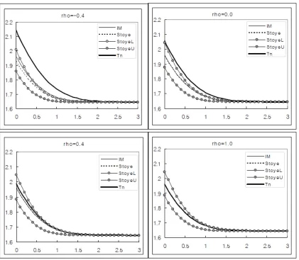
latter two DGPs are presented in Table 2 below.

Table 2: Summary Statistics of DGP2 and DGP3 Brackets Variable # of Values [ l; u] [ l; u]

16 [YL; YU] 13290 [4:4409;4:9059] [1:10;0:861] 0:495 0:4650

The length of the identi…ed interval in the 16 bracket case is eight times smaller than that of

the 2-bracket case. Moreover, the magnitude of in the 16 bracket experiment is almost half of l

and u. So, l and u in the 16 bracket case are close enough for us to expectbn to play a role at

least in small samples. In contrast, in the two bracket case, is large almost twice ofmax_f l; ug.

To implement CIFP and CIS, we need to choose bn. We used bn = s:d: ^ c=ln (n) with

c _{2 f}0;3:5;4_g. When c= 0, bn = 0 which does not satisfy our conditions on bn in Theorem 2.1.

We chose thisbn to illustrate two points. First, when the parameter 0 is point identi…ed or when

is small, it’s possible that bl is larger than bu in which case, the e¤ect of using the shrinkage

estimator with bn = 0 is to replace negative b’s with zero; Second, when is large enough, the

shrinkage estimator withbn= 0is the same as the original estimator and in this case, we’ll observe

the performance ofCIFP and CIS using the original estimator b. Whenc= 3:5;4,bn satis…es the

conditions of Theorem 2.1,CIFP andCIS are uniformly asymptotically valid and non-conservative

in all cases.

Throughout the simulation, we used = 0:05 and 2000 replications. We compare the …nite

sample performance ofCIFP,CIS, andCIPA via their minimum coverage rates referred to as …nite

sample con…dence sizes, see AG (2007). Given that their asymptotic con…dence sizes are achieved

at either l (hl = 0) or u (hu = 0), we report the respective coverage rates of CIFP, CIS, and

CIPA for = l; u.

4.2.1 Point-Identi…ed Case

We …rst present results for YLi =YU i fori= 1; ::; n. In this case, bl =bu, so b = 0 and all three

CIs are the same given by:

CIn= bl

1:96_bl

p

n ;bl+

1:96_bl

p

n :

This is also the CI of IM and Horowitz and Manski (2000). Its coverage rates denoted by CR( 0)

and width over 2000 simulations are reported in Table 3 below.

Table 3: Summary Statistics forCIn

n CR( 0) Width 500 0:9485 0:1720 1000 0:9525 0:1219 2000 0:950 0:0861 8000 0:9520 0:0431

As expected, the coverage rate is very close to the nominal level (0:95) for all sample sizes

In the second experiment, _fYLign_i=16=fYU ig_in₌₁, even though E[YLi] =E[YU i]. In this case, b

may not be exactly zero. In fact, it is possible that b is negative. Since we drew random samples

fYLig and fYU ig independently, we would expect this to happen at about 50% of the simulations.

In Table 4 below, we presented the proportion of simulations with ^ < bn denoted byP( ). This

is the proportion of simulations in which the shrinkage estimator plays a role. When c = 0,

P( )shows the proportion of simulations with negative b. It is about 0.5 for all sample sizes. In addition, we reported the coverage rates and width of each CI based on each value of bn together

with the average of pc1 denoted as Avg(pc1 )6.

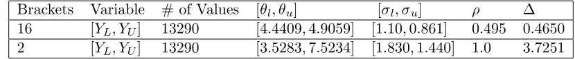
Table 4: Summary Statistics when = 0

n c P( ) Avg(pc1 ) CR( 0) Width

500 CIS 0 0:497 (1:8487;1:8268) 0:9495 0:1619 (3:5;4) 1 (1:9553;1:9558) 0:9495 0:1722

CIFP 0 0:497 1:9087 0:9480 0:1701

(3:5;4) 1 2:0569 0:9480 0:1833

CIPA 2:0569 0:9480 0:1833

1000 CIS 0 0:4945 (1:8476;1:8318) 0:9425 0:1146 3:5;4 1 (1:9546;1:9555) 0:9435 0:1218

CIFP 0 0:4945 1:9110 0:9430 0:1206

(3:5;4) 1 2:0569 0:9445 0:1298

CIPA 2:0569 0:9445 0:1298

2000 CIS 0 0:496 (1:8459;1:8323) 0:9455 0:0806 (3:5;4) 1 (1:9551;1:9547) 0:9455 0:0857

CIFP 0 0:496 1:9101 0:9425 0:0849

(3:5;4) 1 2:0569 0:9425 0:0915

CIPA 2:0569 0:9425 0:0915

8000 CIS 0 0:499 (1:844;1:833) 0:9470 0:0404 (3:5;4) 1 (1:9547;1:9549) 0:9470 0:0430

CIFP 0 0:499 1:9087 0:9480 0:0425

(3:5;4) 1 2:0568 0:9480 0:0458

CIPA 2:0568 0:9480 0:0458

Several conclusions emerge from Table 4: First, the con…dence sizes of all three CIs are almost

the same for all sample sizes and are close to the nominal level, ranging from 0.9421 to 0.9495; Second, the coverage rates of each of CIFP andCIS are almost the same across the three values of

c. The one with c= 0 shows slightly narrower CI than c = 3:5;4; Third, CIFP with c= 3:5;4 is

the same asCIPA, asP( ) = 1 in both cases; Fourth, the critical values in this case are no longer

1.96 as in the case _fYLigni=1 =fYU igni=1, as = 0 in this case.

6_ForCI

4.2.2 Interval-Identi…ed Case

Sixteen Brackets: A small The coverage rates for l and u along with some summary

statistics are presented in Table 5 below.

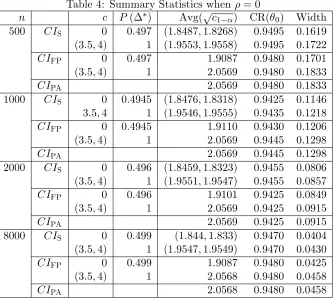
Table 5: Summary Statistics for 16 Brackets

n c P( ) Avg(pc1 ) Width CR( l) CR( u)

500 CIS 0 0 (1:6449;1:6449) 0:6082 0:9235 0:9360 (3:5;4) 1 (1:9024;2:0263) 0:6353 0_:9550 _0:9725

CIFP 0 0 1:6449 0:6082 0:9235 0:9360

(3:5;4) 1 1:9759 0:6371 0_:9595 _0:9655

CIPA 1:9759 0:6371 0:9595 0:9655

1000 CIS 0 0 (1:6449;1:6449) 0:5653 0:9230 0:9340 3:5;4 1 (1:9020;2:0260) 0:5845 0_:9535 _0:9715

CIFP 0 0 1:6449 0:5653 0:9230 0:9340

(3:5;4) 1 1:9760 0:5857 0_:9570 _0:9630

CIPA 1:9760 0:5857 0:9570 0:9630

2000 CIS 0 0 (1:6449;1:6449) 0:5367 0:9335 0:9370 3:5 0:4655 (1:7641;1:8228) 0:5429 0_:9515 _0:9625

4 1 (1:9015;2:0263) 0:5503 0_:9570 _0:9685

CIFP 0 0 1:6449 0:5367 0:9335 0:9370

3:5 0:4655 1:7990 0:5433 0_:9570 _0:9580

4 1 1:9761 0:5512 0:9640 0_:9630

CIPA 1:9761 0:5512 0:9640 0:9630

8000 CIS (0;3:5;4) 0 (1:6449;1:6449) 0:5013 0:9450 0:9435

CIFP (0;3:5;4) 0 1:6449 0:5013 0:9450 0:9435

CIPA 1:9761 0:5086 0:9720 0:9705

In sharp contrast to the point identi…ed case, the con…dence sizes of CIFP andCIS in this case

di¤er signi…cantly for c = 0 and c = 3:5;4. Note that when c = 0, P( ) = 0; so the shrinkage

estimator didn’t play any role in CIFP and CIS. Comparing the con…dence sizes of CIFP and

CIS for c = 0 and c = 3:5, we see clearly the role played by the shrinkage estimator : When

c= 0,P( ) = 0 and both CIFP and CIS under cover except when n= 8000, but when c= 3:5;

P( ) = 1forn= 500;1000 and P( ) = 0:4655forn= 2000, the con…dence sizes of bothCIFP

andCIS are closer to 0.95. Whenc= 4; P( ) = 1 forn= 500;1000;2000and the con…dence size

of CIFP is the same as that ofCIPA. When n= 8000; P( ) = 0for all c and the con…dence size

of both CIFP and CIS is 0:9435 as opposed to 0:9705 for CIPA, con…rming the non-conservative

nature ofCIFP andCIS. In general the width of CIFP is slightly larger than that of CIS.

It is very interesting to compare the con…dence sizes ofCIFP forc= 0 acrossn. For alln,CIFP

large enough for the asymptotics to take e¤ect leading to smaller con…dence size. In contrast, when

n= 8000,pn is large enough leading to the con…dence size of0:9435, the same as the con…dence

size for c = 3:5;4. These results demonstrate clearly the role of c or bn when pn is not large

enough (see n= 500, e.g.): increase the critical values so as to correct the con…dence size. When

p

n is large enough, c or bn is no longer e¤ective and the asymptotics kick in.

Two Brackets: A large In this case, pn is large enough for all sample sizes considered

and bn does not play any role, i.e.,P( ) = 0 for all cand all sample sizes.

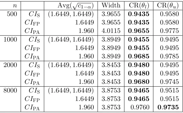
Table 6: Summary Statistics for Two Brackets

n Avg(pc1 ) Width CR( l) CR( u)

500 CIS (1:6449;1:6449) 3:9655 0:9435 0:9580

CIFP 1:6449 3:9655 0:9435 0:9580

CIPA 1:960 4:0115 0:9655 0:9775

1000 CIS (1:6449;1:6449) 3:8949 0:9455 0:9495

CIFP 1:6449 3:8949 0:9455 0:9495

CIPA 1:960 3:8949 0:9685 0:9785

2000 CIS (1:6449;1:6449) 3:8453 0:9480 0:9495

CIFP 1:6449 3:8453 0:9480 0:9495

CIPA 1:960 3:8453 0:9680 0:9745

8000 CIS (1:6449;1:6449) 3:8753 0:9465 0:9515

CIFP 1:6449 3:8753 0:9465 0:9515

CIPA 1:960 3:8753 0:9760 0:9735

The …rst observation from Table 6 is that CIS and CIFP are identical with con…dence size

being very close to the nominal level 0.95 for all sample sizes. However, CIPA is quite di¤erent

from CIS and CIFP: it overcovers for all sample sizes. Secondly, the critical value for CIPA is 1_{(1 =2) = 1:96;because^ = 1; while that forCI}

S and CIFP is 1(1 ) = 1:645, because

p

n is large enough for all sample sizes considered.

5

Conclusion and Current Research

In this paper, we provided a detailed theoretical and numerical study on CIs for interval identi…ed

parameters. By inverting a two-sided test for the value of the interval identi…ed parameter, we

not only developed a new CI, but also established its relationship with existing CIs, including

that of IM, Horowitz and Manski (2000), Stoye (2007), and AG (2007). This approach allows

straightforward extensions to interval identi…ed parameters for which the estimators of the interval

bounds are not asymptotically normally distributed, provided they do not have discontinuity as a

parameters to parameters de…ned by general moment equalities/inequalities.

The simulation results presented in this paper support the theoretical …nding of Stoye (2007)

and the current paper: it is essential to use the shrinkage estimator of the length of the identi…ed

interval or that of the slackness parameters in the general case of parameters de…ned by moment

equalities/inequalities. The shrinkage estimator essentially distinguishes between binding and

non-binding moment inequalities.

The CI or CS developed in this paper has applicability in a wide range of economic/econometric

models with partially identi…ed parameters. Moreover, the idea underlying them can be extended

to partially identi…ed models for which at least one of the assumptions in this paper is violated. For

example, the validity ofCIFP relies on the assumption that the asymptotic distribution of bl;bu

does not have a discontinuity in the model parameters. This may be violated in some applications.

One of the authors is currently working on two such applications.

Park (2007a) investigates inference for the distribution of the treatment e¤ects of a binary

treatment. Using the same notation as in Example 2, but de…ne 0 =F ( ), l= supymax(F1(y)

F0(y );0) and u = 1 + infymin(F1(y) F0(y );0). Then it is known that l 0 u.

Again, with randomized data, F1 and F0 are identi…ed and thus l, u are identi…ed. Estimators

of l; u can be constructed by replacing F1 and F0 with their consistent estimators such as the

empirical distributions in the above expressions. However, the estimators of l; u do not satisfy

Assumption IM (i), as their asymptotic distribution exhibits discontinuity depending on the value

ofsup_y(F1(y) F0(y ))and infy(F1(y) F0(y )). Fan and Park (2007b) considered inference

on the bounds themselves.

Another example violating Assumption IM (i) concerns the ‘mixing problem’ discussed by

Man-ski (1997, 2003). The ‘mixing problem’ arises, for example, when we want to “extrapolate the results

from a randomized experiment,” see Manski (2003). Since we do not know the ‘treatment shares,’

i.e., the possibility that people comply the rule and do not, the probability for a certain range of

out-comes, sayy₂B, to occur lies in[max_fP1(y2B) +P0(y2B) 1;0g;minfP1(y2B) +P0(y2B);1g],

wherePj; j = 1;0;is the probability measure corresponding toFj. Park (2007c) studies the

statis-tical inference for this problem and provides some empirical applications.

Park (2007b) provides an application of the tools developed in Fan and Park (2007b) and Park

(2007a, 2007c) to the Project STAR. Project STAR, conducted by Tennessee State Department of Education in 1985-1988, is a randomized experiment to investigate the e¤ect of class size reduction

(CSR) on students’ performances. Although the potential heterogeneity of treatment e¤ects of

Project STAR has been documented in the literature (see e.g., Ding and Lehrer 2005), it has not

6

Appendix A: Technical Proofs

For convenience, we restate the assumptions (3.3) in AG (2007) as Assumption MI below.

Assumption MI. For i.i.d. observations, the parameter space for ( ; P)is the set of all( ; P)

that satisfy:

(i) Emj(Wi; 0) 0 forj= 1; :::; p;

(ii) Emj(Wi; 0) = 0 forj=p+ 1; :::; k;

(iii) _fWigni=1 are i.i.d.,

(iv) 2

j( )2(0;1) forj= 1; :::; k;

(v) Corr(m(Wi; ))2 , and

(vi) E_jmj(Wi; )= j( )j2+ M forj= 1; :::; k;

where is the set of correlation matrices, and M <₁; >0 are …xed constants.

Proof of Theorem 2.1. Similar to the proof of Theorem 2 in AG (2007), it is straightforward

to show that under Assumption IM (i) and (ii), Assumption A0 and Assumption B0 in AG (2007) are satis…ed withJhthe distribution function of the random variable Zl;h hl ₊2 + Zu;h +hu 2.

Similar to Stoye (2007), we letcn= n 1=2bn

1=2

. Thencn!0andn1=2cn! 1. We consider two

cases: Case I. n cn; Case II. n< cn.

Case I. n cn. In this case, n1=2 n n1=2cn! 1, so eitherhl =1 or hu =1 or both.

Supposehl=1. Then under the local sequence !n;h , we obtain

Pr [ ₂CIFP] = Pr Tn( ) cv1

p

n

max_fbl;bug

;0;_b

! Pr Zl;h hl 2₊+ Zu;h +hu 2 cv1

p

n

max_fbl;bug

;0;_b

! Pr Zu;h +hu 2 cv1

p_n

max_fbl;bug

;0;_b

! Prh Zu;h +hu 2 cv1 (1;0; )

i

Prh(Zu; )2 cv1 (1;0; )

i

1 ,

where we have used the result that the random variable Zu;h +hu 2 is stochastically decreasing

inhu 0 and the result that Pr

h

= bi_!1 because Prhb > bn

i

!1. The proof for hu =1

Case II. n < cn. In this case, Stoye (2007) shows that = 0 with probability

approaching one. Note that under the local sequence _!n;h ,

Pr [ ₂CIFP] = Pr Tn( ) cv1

p

n

max_fbl;bug

;0;_b

! Pr Zl;h hl 2₊+ Zu;h +hu 2 cv1

p_n

max_fbl;bug

;0;_b

! Prh Zl;h hl 2₊+ Zu;h +hu 2 cv1 (0;0; )

i

Prh Zl;h 2₊+ Zu;h 2 cv1 (0;0; )

i

= 1 ,

where we have used the result that the random variable Zl;h hl 2₊+ Zu;h +hu 2 is

sto-chastically decreasing in hl 0; hu 0. The proof is completed by noting that when = 0,

Pr [ ₂CIFP]!1 .

Proof of Theorem 3.1. We prove the result whenp= 2. The general case is similar. Similar

to the proof of Theorem 2.1, we need to justify the use of ₁( ) = _1;1( ); _1;2( ) , where

1;j( ) =

( _m

n;j( )

bn;j( ) ifmn;j( )> bn

0 otherwise :

Letcn= n 1=2bn

1=2

. Then cn!0 andn1=2cn! 1.

Case I. _1;j( ) cn, j = 1;2. In this case, n1=2 1;j( ) n1=2cn! 1. Thus,

Pr ( ₂CSMC) ! Pr

0 @

p+v

X

j=p+1

Zh2;2;j

2

cv1 (1;1; n( ))

1 A

= 1 :

Case II. _1;j( )< cn, j= 1;2. Similar to Stoye (2007), one can show that 1;j( ) = 0 1;j

with probability approaching one. Thus,

Pr ( ₂CSMC) _! Pr

0 @

p

X

j=1

Zh2;2;j+h1

2 +

p+v

X

j=p+1

Zh2;2;j

2

cv1 (0;0; n( ))

1 A

Pr

0 @

p

X

j=1

Zh2;2;j

2 +

p+v

X

j=p+1

Zh2;2;j

2

cv1 (0;0; n( ))

1 A

= 1 :

0 _1;1 with probability approaching one and n1=2

1;2( ) n1=2cn! 1. Thus,

Pr ( ₂CSMC) ! Pr

0 @

p

X

j=1

Zh2;2;j+h1

2 +

p+v

X

j=p+1

Zh2;2;j

2

cv1 (0;1; n( ))

1 A

Pr

0 @ Zh2;2;1

2 +

p+v

X

j=p+1

Zh2;2;j

2

cv1 (0;1; n( ))

1 A

= 1 :

The proof is completed by noting that when all the inequalities are binding, Pr ( ₂CSMC)!

1 .

7

Appendix B: An Expression for

J

₍

x

₎

In this section, we derive a closed-form expression for Jh(x). This should be useful in

construct-ing CSs in moment inequality models when there are two moment constraints. Let (zl; zu; )

and (zl; zu; ) denote respectively the pdf and cdf of (Zl; ; Zu; ): the standard bivariate normal

distribution with correlation coe¢cient . De…ne

A1(x) = (zl; zu)2R2 :zl< hl^zu > hu ;

A2(x) = (zl; zu)2R2 :zl< hl^ hu px zu hu ;

A3(x) = (zl; zu)2R2 :hl zl hl+px^zu> hu ;

A4(x) =

n

(zl; zu)2R2:hl zl hl+px^ hu px zu hu^(zl hl)2+ (zu+hu)2 x

o

;

A(x) = A1(x)[A2(x)[A3(x)[A4(x):

If_{j j}<1, then

Jh(x) = J(hl;hu; )(x)

= P (Zl; hl)₊2 + (Zu; +hu)2 x

= P((Zl; ; Zu; )2A1(x)[A2(x)[A3(x)[A4(x))

=

Z ₁

1

Z ₁

1

I_f(zl; zu)2A(x)g (zl; zu; )dzldzu;

Hence,

Jh(x) = Pr

h

(Zl; hl)2₊+ (Zu; +hu)2 x

i

= hl+px hl; hu px

Z hl+px

hl

Z hu q

x (zl; hl) 2

1

(zl; zu; )dzudzl

= hl+px

Z hl

1

(z) z+hu+

p

x

p

1 2

!

dz

Z hl+px

hl

(z)

0

@ z+hu+ q

x (z hl)2

p

1 2

1 Adz

= hl+px

Z hl+px

1

(z)

0

@ z+hu+ q

x (z hl)2+

p

1 2

1 Adz:

If = 1, then

n

(Zl; hl)2₊+ (Zu; +hu)2 x

o

=nZ : (Z hl)2++ (Z+hu) 2

xo,

whereZ is a standard normal random variable. A similar analysis shows that

n

Z : (Z hl)2++ (Z+hu)2 x

o

= hl < Z hl+px [ hu px Z < hu [ f hu Z hlg

= hu px < Z hl+px :

Therefore, we get

J(hl;hu;1)(x) = Pr (Zl; hl)

2

++ (Zu; +hu) 2 _x

If = 1, then

Pr (Zl; hl)2₊+ (Zu; +hu)2 x = Pr (Z hl)2++ ( Z+hu)2 x

= Pr (Z hl)2++ (Z hu)2+ x :

Letmax_fhl; hug=hmaxandminfhl; hug=hmin. We can rewrite the event

n

(Z hl)2++ (Z hu) 2 + x

o

as:

n

(Z hl)2++ (Z hu)2+ x

o

=B1(x)[B2(x)[B3(x)[B4(x);

where Bj(x), j = 1;2;3;4 correspond to the four possibilities in terms of the signs of (Z hl);

(Z hu). For example,

B1(x) =

n

Z :Z hl>0^Z hu >0^(Z hl)2₊+ (Z hu)2₊ x

o

:

Note thatZ hl>0 and Z hu >0 is equivalent toZ > hmax. In this case,

n

Z : (Z hl)2++ (Z hu)2+ x

o

=

(

Z : Z hl+hu

2

2 _{2x (h}

l hu)2

4

)

=

8 < :Z :Z

hl+hu+

q

2x (hl hu)2

2

9 =

; provided2x (hl hu)

2

=

8 < :Z :Z

hmax+hmin+

q

2x (hmax hmin)2 2

9 =

; provided2x (hmax hmin)

2_:

Also,

hmax<

hmax+hmin+

q

2x (hmax hmin)2

2 =) (hmax hmin) 2_{< x:}

Therefore, we get

B1(x) =

8 < :

Z :hmax< Z hmax+hmin+

p

2x (hmax hmin)2

2 ifx >(hmax hmin)

2

;

? _otherwise

Similarly, we can show:

B2(x) = Z:hmin Z <min hmax; hmin+px

B3(x) = Z:hmin Z <min hmax; hmin+px

Combining them altogether, we get

n

(Z hl)2++ (Z hu)2+ x

o

= ₁;min hmax; hmin+px [

8 < :

?_{ifx (hmax hmin)}2

hmax;hl+hu+

p

2x (hmax hmin)2

2 otherwise

=

8 < :

( ₁; hmin+px) ifx (hmax hmin)2

1;hl+hu+

p

2x (hmax hmin)2

2 otherwise

Therefore,

Pr (Zl; hl)2₊+ (Zu; +hu)2 x

=

8 < :

(hmin+px) ifx (hmax hmin)2

hmax+hmin+

p

2x (hmax hmin)2

2 otherwise

:

8

Appendix C. The Forms of

CI

_and

CI

In this section, we show that bothCIPA andCIFP are intervals because their critical values do not

depend on . In general, CSn de…ned as

CSn = f :Tn( ) c1 g

=

8 < : :n

^_l

^l

!2

+

+n ^u

^u !2 c1 9 = ;

with a constant critical value c1 has the following alternative expressions:

CSn=

8 > > > > > > > > > < > > > > > > > > > : h

^_l p_{c1 p}^l

n;^u+

p_c

1 p^u_n

i

ifpnb pc1 minf^l;^ug

h

^

l pc1 p^_nl; B

i

if pc1 ^l pnb <pc1 ^u

h

A;^u+pc1 p^u_n

i

if pc1 ^u pnb <pc1 ^l

[A; B] if qc1 ^2u+ ^2l

p

nb < pc1 maxf^l;^ug

? _ifp_nb _<

q

c1 ^2l + ^2u

(17)

where

A ^

2

u^l+ ^2l^u

^2_u+ ^2_l

v u u

t ^2l^2u

n ^2_u+ ^2_l

"

c1

nb2 ^2_u+ ^2_l

#

;

B ^

2

u^l+ ^2l^u

^2_u+ ^2_l +

v u u

t ^2l^2u

n ^2_u+ ^2_l

"

c1 n

b2 ^2_u+ ^2_l

#