Munich Personal RePEc Archive
An empirical comparison of alternate
regime-switching models for electricity
spot prices
Janczura, Joanna and Weron, Rafal
6 February 2010
Online at
https://mpra.ub.uni-muenchen.de/22876/
An empirical comparison of alternate regime-switching models for electricity
spot prices
Joanna Janczura
Hugo Steinhaus Center, Institute of Mathematics and Computer Science, Wrocław University of Technology, 50-370 Wrocław, Poland
Rafał Weron
Institute of Organization and Management, Wrocław University of Technology, 50-370 Wrocław, Poland
Abstract
One of the most profound features of electricity spot prices are the price spikes. Markov regime-switching (MRS) models seem to be a natural candidate for modeling this spiky behavior. However, in the studies published so far, the goodness-of-fit of the proposed models has not been a major focus. While most of the models were elegant, their fit to empirical data has either been not examined thoroughly or the signs of a bad fit ignored. With this paper we want to fill the gap. We calibrate and test a range of MRS models in an attempt to find parsimonious specifications that not only address the main characteristics of electricity prices but are statistically sound as well. We find that the best structure is that of an independent spike 3-regime model with heteroscedastic diffusion-type base regime dynamics and shifted spike regime distributions. Not only does it allow for consecutive spikes or price drops, which is consistent with market observations, but also exhibits the ‘inverse leverage effect’ reported in the literature for spot electricity prices.
Keywords: Electricity spot price, Spikes, Markov regime-switching, Heteroscedasticity, Inverse leverage effect.
1. Introduction
The valuation of electricity contracts is not a trivial task. If the model is too complex the computational burden will prevent its on-line use in trading departments. On the other hand, if the price process chosen is inappropriate to capture the main characteristics of electricity prices, the results from the model are unlikely to be reliable.
The uniqueness of electricity as a commodity prevents us from simply using models developed for the financial or other commodity markets. Electricity cannot be stored economically and requires immediate delivery, while end-user demand shows high variability and strong weather and business cycle dependence. Effects like power plant outages or transmission grid (un)reliability add complexity and randomness. The resulting spot price series exhibit strong seasonality on the annual, weekly and daily level, as well as, mean reversion, very high volatility and abrupt, short-lived and generally unanticipated extreme price changes known as spikes or jumps.
Despite numerous attempts (for reviews see e.g. Benth et al., 2008; Bunn, 2004; Kaminski, 2004; Weron, 2006), the need for realistic models of price dynamics capturing the unique characteristics of electricity and adequate deriva-tives pricing techniques still has not been fully satisfied. It is the aim of this paper to suggest parsimonious models for electricity spot price dynamics that not only address the main characteristics of electricity prices but are statistically sound as well. The parsimony is a prerequisite of derivatives pricing, especially simulation techniques, where the numerical burden can be substantial. The statistical adequacy, on the other hand, is a requirement in any modeling task.
We focus on Markov regime-switching (MRS) models, which seem to be a natural candidate for modeling the spiky, non-linear behavior of electricity spot prices. In a way, they offer the best of the two worlds; they are a trade-off
between model parsimony and adequacy to capture the unique characteristics of power prices. In contrast to threshold type regime-switching models (like TAR, STAR, SETAR), in MRS models the regimes are only latent. Consequently, MRS models do not require an upfront specification of the threshold variable and level and, hence, are less prone to modeling risk.
Yet, despite this latency, there are still enough ‘free parameters’ in MRS models to make the calibration procedure a tough exercise, even for experienced professionals. Firstly, the number of regimes has to be agreed upon. In almost all published studies only 2-regime models were considered, most likely due to a lower computational burden. Apart from a base regime, a spike (or excited) regime was introduced for modeling the extreme price behavior. However, there is no fundamental reason for not considering 3- or multi-regime specifications. In fact, analyzing UK half-hourly electricity spot prices Karakatsani and Bunn (2008) identified three regimes, with the third regime capturing the most extreme prices. The estimated switching pattern suggested a two-stage spike reversal to normal prices. Also, for many of the very low prices a technical (or fundamental) event underlying the non-standard behavior can be identified, justifying existence of a separate ‘down-spike’ or ‘drop’ regime.
Secondly, the stochastic processes defining the price dynamics in each of the regimes have to be selected. The base regime is typically of a mean-reverting diffusion-type, however, for the spike regime(s) a number of specifications have been suggested, ranging from mean reverting diffusions to heavy tailed random variables.
Finally, the dependence between the regimes has to be decided upon. Dependent regimes with the same random noise process in all regimes (but different parameters) lead to computationally simpler models. On the other hand, independent regimes allow for a greater flexibility and seem to be a more natural choice for a process which, from time to time, radically changes its dynamics.
This paper is intended as a guide to MRS models for spot electricity prices. In Section 2 we present the datasets and explain the deseasonalization procedures. In Section 3 we explain the estimation process and goodness-of-fit testing. Next, in Section 4 we review the first and second generation models and discuss their pros and cons. In Section 5 we calibrate various MRS models to deseasonalized prices and log-prices, evaluate their goodness-of-fit and select the optimal model structure. Finally, in Section 6 we conclude.
2. The datasets
2.1. Three markets, six datasets
In this study we use mean daily (baseload) day-ahead spot prices from three major power markets: the Euro-pean Energy Exchange (EEX; Germany), the PJM Interconnection (PJM; U.S.) and the New England Power Pool (NEPOOL; U.S.). For each market the sample totals 2926 daily observations (or 418 full weeks) and covers the 8-year period January 1, 2001 – January 4, 2009. To see how robust are the presented models and how well they perform under different market conditions each dataset is split into two subsamples of equal length (1463 daily observations or 209 weeks each): January 1, 2001 – January 2, 2005 (EEX1, PJM1 and NEP1) and January 3, 2005 – January 4, 2009 (EEX2, PJM2 and NEP2), see Figures 1-2.
Note, that the different dynamics of spot electricity prices in the second four-year period coincide with a change in market fundamentals. The electricity price hike in 2005 was largely due to higher natural gas (NG) prices. In Europe, the fuel prices were pushed up by the decline in North Sea production and a cold winter of 2005/2006 (Davoust, 2008). The introduction of CO2 emission costs in January 2005 (Benz and Tr¨uck, 2006) added momentum. In the U.S., the
doubling of NG prices was initiated by hurricanes Katrina and Rita which damaged Gulf of Mexico production, pro-cessing and transportation infrastructure. This volatile period was followed by roughly 18 months of more moderate prices and the second ‘fuel bubble’, which started in September/October 2007 and ended in July/August 2008 with the burst of the ‘oil bubble’ (Hamilton, 2009; Khan, 2009).
300 600 900 1200 0
50 100 150 200 250 300
Price [EUR/MWh]
EEX1 [Jan 1, 2001 − Jan 2, 2005]
Price LTSC
300 600 900 1200 0
50 100 150 200 250 300
Price [EUR/MWh]
EEX2 [Jan 3, 2005 − Jan 4, 2009]
Price LTSC
300 600 900 1200 0
5 10 15 20
Price [GBP/mmbtu], Index/100
NG & Coal [Jan 1, 2001 − Jan 2, 2005]
NBP (Natural Gas, UK) NWE Steam Coal Index
300 600 900 1200 0
5 10 15 20
Price [GBP/mmbtu], Index/100
[image:4.595.94.505.116.432.2]NG & Coal [Jan 3, 2005 − Jan 4, 2009]
Figure 1: Mean daily spot prices and their long-term seasonal components (LTSC; thick blue lines) for the EEX power market in Germany (top
panels). The fundamental price drivers – the National Balancing Point (UK) natural gas day-ahead prices and the McCloskey North West Europe Steam Coal Index (rescaled by 100 to fit in the plot) – are shown for comparison in the bottom panels. The NBP prices are quoted in GBP/therm, but have been rescaled to the GBP/mmbtu units to make them more comparable to the Henry Hub prices in Figure 2. The unit mmbtu stands for
one million British thermal unitsor 10therms. The first four years (January 1, 2001 – January 2, 2005) of the study period are presented in the left panels and the latter four years (January 3, 2005 – January 4, 2009) in the right panels.
(NBP) natural gas day-ahead prices in the UK as a proxy for the European NG market. In the U.S. the largest and most important natural gas hub is the Henry Hub in Louisiana. As for the two other fuels, we use the McCloskey North West Europe Steam Coal Index as a proxy of the European coal market and two HWWI indexes – the HWWI World Crude Oil Index and the HWWI World Coal Index – as proxies for the U.S. fuel markets.
The natural gas/electricity price dependence can be seen very well in the period mid-November 2005 – mid-March 2006 (days #310-#445 in the right panels of Figure 1). The sudden increase of European NG prices led to an instant increase of on-peak prices (and hence mean daily prices) in the EEX market. In the U.S., the Henry Hub price spike in late February 2003 (due to a severe cold front that increased demand and reduced supply by freezing-off
producing wells; days #780-#790 in the left panels of Figure 2) caused spikes in PJM and NEPOOL prices, though not necessarily the most severe in history. The influence of all three fuels – NG, oil and coal – on electricity can be seen in the last months of 2008. Due to the sub-prime crisis in the U.S., the global economy went into a recession and the demand for energy products dramatically decreased. The burst of the ‘oil bubble’ in mid-2008 had an immediate effect on the U.S. power markets (PJM and NEPOOL), but a delayed effect on the European power market (EEX). In the latter case, the spot electricity prices dropped irrespective of the relatively constant NBP prices; the falling coal prices eventually led to the price decrease.
300 600 900 1200 0
50 100 150 200 250 300
Price [USD/MWh]
PJM2 [Jan 3, 2005 − Jan 4, 2009]
Price LTSC
300 600 900 1200 0
50 100 150 200 250 300
Price [USD/MWh]
PJM1 [Jan 1, 2001 − Jan 2, 2005]
Price LTSC
300 600 900 1200 0
100 200 300 400
Price [USD/MWh]
NEP2 [Jan 3, 2005 − Jan 4, 2009]
Price LTSC
300 600 900 1200 0
100 200 300 400
Price [USD/MWh]
NEP1 [Jan 1, 2001 − Jan 2, 2005]
Price LTSC
300 600 900 1200 0
5 10 15 20
Price [USD/mmbtu], Index/100
NG, Oil & Coal [Jan 1, 2001 − Jan 2, 2005]
300 600 900 1200 0
5 10 15 20
Price [USD/mmbtu], Index/100
NG, Oil & Coal [Jan 3, 2005 − Jan 4, 2009]
[image:5.595.91.510.163.637.2]H.Hub (Natural Gas, USA) HWWI World Crude Oil Index HWWI World Coal Index
the strategic bidding practices, which at times significantly change the spot prices. Having all this in mind and not wanting to focus the paper on modeling the fuel stack/bid stack/electricity spot price relationships we will use a single non-parametric long-term seasonal component (LTSC) to represent the long-term non-periodic fuel price levels, the changing climate/consumption conditions throughout the years and strategic bidding practices. As can be seen in Figures 1-2, the LTSC – obtained by wavelet smoothing of electricity spot prices (see the next Section for details) – pretty well reflects the ‘average’ fuel price level, understood as a combination of NG, crude oil and coal prices.
2.2. Deseasonalization
There are different suggestions in the literature for dealing with the seasonal pattern in electricity price dynamics. Here we follow the ‘industry standard’ and represent the spot pricePt by a sum of two independent parts: a (pre-dictable) seasonal component ftand a stochastic componentXt, i.e. Pt = ft+Xt. Further, we let ftbe composed of a weekly periodic partst and a long-term seasonal componentTt, which represents the long-term non-periodic fuel price levels, the changing climate/consumption conditions throughout the years and strategic bidding practices.
As in Weron (2009) the deseasonalization is conducted in three steps. First,Ttis estimated from daily spot prices
Pt using a wavelet filtering-smoothing technique (for details see Tr¨uck et al., 2007; Weron, 2006). Recall, that any function or signal (here: Pt) can be built up as a sequence of projections onto one father wavelet and a sequence of mother wavelets:SJ+DJ+DJ−1+...+D1, where 2Jis the maximum scale sustainable by the number of observations.
At the coarsest scale the signal can be estimated bySJ. At a higher level of refinement the signal can be approximated bySJ−1=SJ+DJ. At each step, by adding a mother waveletDjof a lower scalej=J−1,J−2, ..., we obtain a better
estimate of the original signal. This procedure, also known as lowpass filtering, yields a traditional linear smoother. Here we use theS8approximation, which roughly corresponds to annual (28=256 days) smoothing, see the thick blue
lines in Figures 1-2. The price series without the LTSC is obtained by subtracting theS8approximation fromPt. Next,
the weekly periodicitystis removed by applying the moving average technique (see e.g. Brockwell and Davis, 2002; Weron, 2006) and subtracting the resulting ‘mean’ weekly pattern. Finally, the deseasonalized prices, i.e.Pt−Tt−st, are shifted so that the minimum of the new process is the same as the minimum ofPt(the latter alignment is required if log-prices are to be analyzed). The resulting deseasonalized time seriesXtcan be seen in Figure 8.
Before we start modeling the stochastic components, two important facts should be mentioned for clarity. Firstly, in terms of smoothing properties wavelet filters show some resemblance to kernel density estimators (KDE). In fact, a KDE with a Gaussian kernel and standard deviation of ca. 90 days yields seasonal components similar to the wavelet estimated LTSC in Figures 1-2. However, unless a complicated local bandwidth choice is employed, KDE are not locally adaptive and for datasets with seasonal components of varying in time frequencies and amplitudes, like electricity spot prices, the bandwidth is typically either too small or too large. Wavelet filters do not share this drawback and, in general, are superior to KDE (H¨ardle et al., 1998).
Secondly, while wavelets offer a very good in-sample fit to the data, their ability to forecast past the near future is rather bad (Ramsey, 2002). A very small number of wavelet coefficients are typically needed to provide good fits to any historical data, but the set of relevant coefficients varies period by period. The reason for this is that individual wavelet functions are localized in time, i.e. the mass of oscillations is concentrated on a small time interval. Consequently, the functions (time series) that are represented by wavelets do not have to be homogeneous over time. This is quite unlike sines and cosines. Fourier analysis assumes that the signal is homogeneous over time, that over any subinterval of the observed time series the precise same frequencies hold at the same amplitudes. This property makes trigonometric representations suitable for forecasting ... at the cost of offering a generally poor in-sample fit. One might argue that the latter can be corrected for by including a smoothing component, like in De Jong (2006), where a sine function is combined with an Exponentially-Weighted Moving Average (EWMA). But this approach essentially boils down to smoothing the prices with a KDE, a wavelet filter or the EWMA itself.
curves in electricity markets (Benth et al., 2007; Borak and Weron, 2008; Fleten and Lemming, 2003) we might be able to forecast the LTSC with a decent accuracy. But if this is the right approach has yet to be tested.
3. Statistical inference for MRS models
3.1. Basic properties
The underlying idea behind the Markov regime-switching (MRS) scheme is to model the observed stochastic behavior of a specific time series by two (or more) separate phases or regimes with different underlying processes. In other words, the parameters of the underlying process may change for a certain period of time and then fall back to their original structure. The switching mechanism between the states is Markovian and is assumed to be governed by an unobserved (latent) random variable. The underlying processes, though, do not have to be Markovian, but are often assumed to be independent from each other.
In the simplest case of a 2-regime model, the spot price can be assumed to display either normal or very high prices (or spikes) at each point in time, depending on the regimeRt =b(‘base’) orRt =s(‘spike’). Consequently, we have a probability law that governs the transition from one state to another. The transition matrixPcontains the probabilitiespi jof switching from regimeiat timetto regime jat timet+1:
P=(pi j)= pbb pbs psb pss
!
= 1−pbs pbs psb 1−psb
!
. (1)
In the more general case of a 3-regime model, the transition matrixPtakes the form:
P=(pi j)=
pbb pbs pbd
psb pss psd
pdb pds pdd
, with pii=1−X
j,i
pi j. (2)
The subscripts{b,s,d}represent the ‘base’, ‘spike’ and ‘drop’ (‘downward spike’) regimes, respectively.
Because of the Markov property the current stateRtat timetof a Markov chain depends on the past only through the most recent valueRt−1. Consequently the probability of being in state jat timet+mstarting from stateiat timet
is given by
P(Rt+m= j|Rt=i)=(P′)m·ei, (3) whereP′denotes the transpose ofPande
idenotes theith column of the identity matrix.
3.2. Calibration
Calibration of MRS models is not straightforward since the regime is only latent and hence not directly observable. Here we follow Hamilton (1990), Kim (1994) and Janczura and Weron (2010a) and apply a variant of the Expectation-Maximization (EM) algorithm. This is an iterative two-step procedure which starts with computing the conditional probabilitiesP(Rt = j|x1, ...,xT;θ) for the process being in regime jat timet, based on starting values ˆθ(0) for the
parameter vectorθof the underlying stochastic processes. These probabilities are referred to as ‘smoothed inferences’. Then, in the second step, new and more exact ML estimates ˆθfor all model parameters are calculated using the smoothed inferences from step one. With each new vector ˆθ(n) the next cycle of the algorithm is started in order to reevaluate the smoothed inferences. Every iteration of the EM algorithm generates new estimates ˆθ(n+1), as well as, new estimates for the smoothed inferences. Each iteration cycle increases the log-likelihood function and the limit of this sequence of estimates reaches a (local) maximum of the log-likelihood function.
It is interesting to note, that if the regimes are independent from each other, then during a spike (or a drop) the base regime becomes latent. If it is defined by an autoregressive process (as in the majority of models considered in the literature), then the calculation of the base regime density – which is used in both steps of the iterative procedure – requires storing the whole set of probabilitiesP(Rt = it,Rt−1 = it−1, ...,R1 = i1). Obviously, this leads to a high
their expectationsE(Xt,b|x1, ...,xt). The subscripts inXt,bdenote the time and regime, respectively. These expectations can be obtained from the following recursive formula:
E(Xt,b|x1, ...,xt)=xtP(Rt=b|x1, ...,xt)+E(g(X1,b, ...,Xt−1,b, ǫ1, ..., ǫt−1)|x1, ...,xt−1)P(Rt,b|x1, ...,xt),
where the functiong(X1,b, ...,Xt−1,b, ǫ1, ..., ǫt−1)=Xt,bdefines the base regime dynamics (as formula (5) in the case of the mean-reverting AR(1) process) andǫ1, ..., ǫt−1is a white noise sequence. The main advantage of this procedure is
efficiency – it requires storing probabilities concerning the last observed price only, as opposed to the last 10 prices in the Huisman and de Jong (2003) approach.
3.3. Goodness-of-f t
We evaluate the adequacy of the models on the base of descriptive statistics, as well as, a goodness-of-fit hypothesis test. The former include the Inter-Quartile and the Inter-Decile Range, i.e. the difference between the third and the first quartiles (IQR) or ninth and first deciles (IDR). The quantile-based measures rather than the less robust to outliers moment-related statistics are used. Furthermore, we report thep-values of the Kolmogorov-Smirnov goodness-of-fit test (K-S test) measuring the difference between the empirical (sample) and theoretical (model implied) marginal distributions. Since the K-S test cannot be applied directly to prices (or log-prices) as they are not i.i.d. in the considered models, following Janczura and Weron (2010b) we transform the data using the smoothed inferences and obtain a mixture of i.i.d. samples resulting from the two (or three) regimes. The K-S test is then performed for the regimes, as well as, for the whole sample.
4. Overview of MRS models for spot electricity prices
4.1. First generation models
To our best knowledge, the MRS models were first applied to electricity prices in Deng (1998) and Ethier and Mount (1998). Deng (1998) considered three models of spot price dynamics in a derivatives pricing context (formal parame-ter estimation was not performed). These included a 2-state regime-switching specification for the log-prices in which the base regime was driven by an autoregressive process of order one, i.e. AR(1), and the spike regime by the same AR(1) process (i.e. with the same parameters) shifted by an exponentially distributed random variable (spike/jump size). In a parallel paper Ethier and Mount (1998) proposed a 2-state model with mean-reverting AR(1) processes for the log-prices in both regimes. The processes shared the same set of random innovations – only the parameters of the two AR(1) processes varied between the regimes. Strong empirical support for the existence of different means and variances in the two regimes was found for data from four U.S. and Australian markets. A similar model was later used by Heydari and Siddiqui (2010) in a gas-fired power plant valuation problem in the UK market, but was found inferior to mean-reverting stochastic volatility models over long-term forecast periods.
Huisman and Mahieu (2003) proposed a regime-switching model with three possible states in which the initial jump regime was immediately followed by the reversing regime and then moved back to the base regime, i.e. with
psd = pdb =1 in (2). Andreasen and Dahlgren (2006) studied a similar MRS model – in their model the spot price could jump up or down if it was in the neutral state (base regime) and it could only jump back to its neutral state if it was in one of the jump regimes. Consequently, these models did not allow for consecutive high prices (in fact of log-prices) and, hence, did not offer any obvious advantage over jump-diffusion models.
This restriction was relaxed by Huisman and de Jong (2003), who proposed a simple independent spike (IS) 2-regime model for deseasonalized log-prices. The base 2-regime was modeled by a mean-reverting AR(1) process and the spike regime by a normal distributed random variable whose mean and variance were higher than those of the base regime process. The third regime was not needed to pull prices back to stable levels, because the prices were independent from each other in the two regimes. Kosater and Mosler (2006) reported that for EEX 2000-2004 data the IS 2-regime model outperformed the model of Ethier and Mount (1998) in terms of short/medium-term forecasts (up to 1 month), while the opposite was true for long-term forecasts. They were able to improve the forecasts if the spike regimes in these models had two sets of parameters – one for business days and one for holidays.
better models for deseasonalized Nord Pool log-prices from the period 1997-2000. This was not the case, as the Pareto distribution seemed to overestimate the spike sizes. The best model (in terms of the likelihood) turned out to be the one with log-normal spikes, closely followed by the model of Huisman and de Jong (2003), i.e. with Gaussian spikes. The 3-regime model of Huisman and Mahieu (2003) came in last.
De Jong (2006) proposed another modification of the basic IS 2-regime model with autoregressive, Poisson driven spike regime dynamics (a similar model was later considered by Mari, 2008). Using 2001-2006 data from eight European and U.S. power markets he compared it to several spot price models. On average the new model yielded the best fit (again in terms of the likelihood), but the IS 2-regime model with Gaussian spikes was nearly as good. Like in the previously mentioned study, the 3-regime model of Huisman and Mahieu (2003) yielded a significantly worse fit, comparable to that of a mean-reverting jump diffusion (MRJD) and slightly worse than that of the threshold model of Geman and Roncoroni (2006). In a related study Bierbrauer et al. (2007) introduced an IS 2-regime model with exponentially distributed spikes. For 2000-2003 EEX market data they found it inferior to MRS models with normal or log-normal spikes, but much better than the non-linear mean-reverting model of Barlow (2002) or the MRJD model of Kluge (2006) with two different mean-reversion rates for the normal and the jump parts.
The main problem with the discussed above first generation models is that they possess a critical flaw. Namely, they do not classify the regimes correctly. This flaw, in many cases, leads to negative ‘expected spike sizes’, i.e.
E(Xt,s) < E(Xt,b), and a significant discrepancy between the often bimodal empirical distribution of (log-)prices classified as spikes and the unimodal theoretical spike distribution, see Figures 3 and 4. Modeling prices themselves instead of log-prices (as proposed by Weron, 2009) generally eliminates the unwanted feature of negative ‘expected spike sizes’. However, still some of the low prices are classified as being in the spike regime, see the lower left panel in Figure 3. The lower number of ‘sudden drops’ classified as spikes suggests that the calibration scheme does a better job of identifying the spikes in prices than in log-prices. But the classification is far from perfect.
4.2. Second generation models
The above mentioned first generation models have two common features. Firstly, not the prices themselves, but rather log-prices are considered. Secondly, the base regime (and in some cases the spike regime as well) is driven by a mean-reverting diffusion process of the form:
dXt,b=(α−βXt,b)dt+σbdWt=β
α β−Xt,b
!
dt+σbdWt, (4)
whereWt is the Brownian motion (i.e. a Wiener process), α
β is the long term mean reversion level,βis the speed of mean reversion and σb is the volatility. In the fixed income literature this popular process is known as the Vasicek (1977) model, in mathematics as the (generalized) Ornstein-Uhlenbeck process (Janicki and Weron, 1994), while in signal processing – when discretized – as an AR(1) process or an autoregressive time series of order one (Brockwell and Davis, 2002):
Xt,b =α+(1−β)Xt−1,b+σbǫt, (5) whereǫthas the standard Gaussian distribution.
But is this the right choice for the base regime dynamics? Should we model prices or log-prices? What about the regime-switching mechanism – perhaps we could use fundamental information to improve the fit? The second generation models try to address some of the deficiencies of the first generation models. They can be grouped into two categories: (i) those that use fundamental information (system constraints, weather variables) to better model regime-switching and (ii) those that propose statistical refinements (to ultimately improve the goodness-of-fit).
In the first group, Mount et al. (2006) proposed a 2-regime model with two AR(1) regimes for log-prices and transition probabilities dependent on the reserve margin. Using PJM data from 1999-2000 they showed that the estimated switching probability from the base (low) to the spike (high) regime predicts price spikes well if the reserve margin is measured accurately. This is in line with the qualitative findings of Kanamura and ¯Ohashi (2008), who showed that the transition probabilities cannot be constant, but depend on the current demand level relative to the supply capacity, the deterministic trend of demand change, and the trend generated by the deviation of temporary demand fluctuation from its long-term mean.
300 600 900 1200 2
3 4 5 6
PJM1 [Jan 1, 2001 − Jan 2, 2005]
Log−price [USD/MWh]
Base Spike
300 600 900 1200 0
0.5 1
P(S)
300 600 900 1200 1
2 3 4 5 6
EEX2 [Jan 3, 2005 − Jan 4, 2009]
Log−price [EUR/MWh]
Base Spike
300 600 900 1200 0
0.5 1
P(S)
300 600 900 1200 0
100 200 300
EEX1 [Jan 1, 2001 − Jan 2, 2005]
Price [EUR/MWh]
Base Spike
300 600 900 1200 0
0.5 1
P(S)
300 600 900 1200 2
3 4 5 6
NEP1 [Jan 1, 2001 − Jan 2, 2005]
Log−price [USD/MWh]
Base Spike
300 600 900 1200 0
0.5 1
[image:10.595.95.503.115.425.2]P(S)
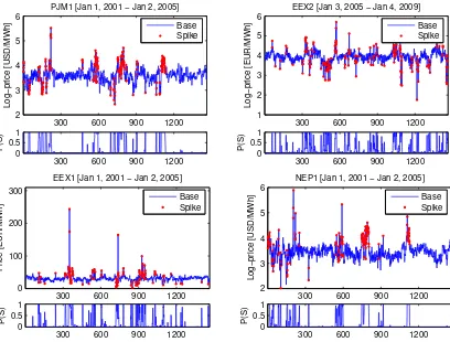
Figure 3: Sample calibration results for 2-regime models with Vasicek, i.e. AR(1), base regime dynamics and alternative spike regimes fitted to deseasonalized prices or log-prices from three major power markets. Top left: An independent spike (IS) model with normal spikes fitted to PJM log-prices.Top right: The Ethier and Mount (1998) model with AR(1) spike regime fitted to EEX log-prices. Bottom left and right: An IS model with lognormal spikes fitted to EEX prices and NEPOOL log-prices, respectively. The corresponding lower panels display the probability
P(S)≡P(Rt=s) of being in the spike regime. The prices or log-prices classified as spikes, i.e. withP(S)>0.5, are additionally denoted by dots in the upper panels. For descriptions of the datasets see Section 2 and Figures 1-2.
from the years 2000-2003 they concluded that the model performed better when modeling the seasons where the planned outages were known. In a non-MRS context, studying the 2003-2006 data for the England and Wales market, Cartea et al. (2009) reached similar conclusions. They showed that the incorporation of forward looking information on capacity constraints significantly improved the modeling of spikes, both timing and magnitude.
In a complementary study to Mount et al. (2006), Huisman (2008) noted that the availability (to every market participant) of the reserve margin data is limited. Hence, he proposed to use temperature as a proxy. Interpreting the results from three MRS models fitted to the Dutch APX log-prices from the period 2003-2008, Huisman showed that the probability of spike occurrence increases when temperature deviates substantially from mean temperature levels. However, in general, temperature does not provide as much information as the reserve margin.
In the second group of models the focus has been on refining the statistical tools used for describing the dynamics of electricity prices. Examples range from non-orthodox approaches originating in physics to more ‘traditional’ econometric ones. For instance, Lucheroni (2009) suggested to model a seasonally and irregularly peaking price dynamics using a FitzHugh–Nagumo system of coupled nonlinear stochastic differential equations. The rationale behind this approach stems from the fact that second order dynamics is obviously richer than first order (like in autoregressions). It can sustain oscillations even without periodic driving, and, when driven, its behavior can be very complex.
−4 −2 0 2 4 0
0.1 0.2 0.3 0.4
Log−price [EUR/MWh]
EEX2 [Jan 3, 2005 − Jan 4, 2009]
Empirical Theoretical
2 3 4 5 6
0 0.2 0.4 0.6 0.8 1
Log−price [USD/MWh]
PJM1 [Jan 1, 2001 − Jan 2, 2005]
Empirical Theoretical
0 50 100 150 200 250 0
0.005 0.01 0.015 0.02 0.025
Price [EUR/MWh]
EEX1 [Jan 1, 2001 − Jan 2, 2005]
Empirical Theoretical
1 2 3 4 5 6 7
0 0.2 0.4 0.6 0.8 1
Log−price [USD/MWh]
NEP1 [Jan 1, 2001 − Jan 2, 2005]
[image:11.595.94.503.119.447.2]Empirical Theoretical
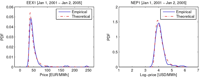
Figure 4: Comparison of empirical (sample) and theoretical (model implied) spike regime probability distribution functions in the first generation 2-regime models. The models and datasets are the same as in Figure 3. Note, that for the Ethier and Mount (1998) model the distributions of the noise in the AR(1) process driving the spike regime are plotted (top right).
were elegant, their fit to empirical data has either been not examined thoroughly or the signs of a bad fit ignored. To eliminate the unwanted feature of negative ‘expected spike sizes’ Weron (2009) proposed to build models not for log-prices, but prices themselves. In a follow up paper Janczura and Weron (2009) tested IS 2-regime models for electricity spot prices with Vasicek and CIR-type (see Cox et al., 1985) dynamics for the base regime and median-shifted spike regime distributions. For EEX market data from the period 2001-2009 they found that models with shifted spike regime distributions (which assign zero probability to prices below the median price) led to more realistic descriptions of electricity spot prices and that by introducing CIR-type heteroscedasticity in the base regime – in place of the standard mean-reverting, constant volatility dynamics – better spike identification was obtained.
Table 1: Goodness-of-fit statistics for 2-regime models with Vasicek, see eqns. (4)-(5), base regime dynamics and median-shifted lognormal or Pareto spike distributions. Models for prices are summarized in columns 2-7, for log-prices in columns 8-13. p-values of 0.05 or more are emphasized in bold.
Prices Log-prices
Simulation K-S test p-value Simulation K-S test p-value Data IQR IDR LogL Base Spike Model IQR IDR LogL Base Spike Model
Shifted lognormal spikes
EEX1 9% 11% -4193.7 0.0012 0.4061 0.0032 30% 30% 403.0 0.0000 0.7371 0.0000 EEX2 13% 3% -5066.9 0.0090 0.4732 0.0149 27% 16% 399.6 0.0000 0.6313 0.0000 PJM1 9% -1% -4385.9 0.0341 0.4346 0.0530 19% 8% 777.4 0.0007 0.3219 0.0012 PJM2 -3% 3% -5012.1 0.0887 0.9196 0.0893 3% 6% 780.1 0.0747 0.4147 0.0696
NEP1 2% 2% -4327.1 0.0247 0.5093 0.0561 9% 8% 610.4 0.0002 0.8316 0.0003 NEP2 0% -2% -4665.9 0.0823 0.8416 0.1251 8% 0% 1417.9 0.0088 0.7430 0.0170
Shifted Pareto spikes
EEX1 7% 9% -4218.6 0.0000 0.0000 0.0000 27% 27% 436.9 0.0000 0.0123 0.0000 EEX2 10% 1% -5101.8 0.0188 0.0008 0.0412 26% 16% 374.6 0.0000 0.0166 0.0000 PJM1 8% -5% -4447.2 0.0500 0.0000 0.0500 20% 6% 755.2 0.0007 0.0000 0.0012 PJM2 0% 1% -5161.6 0.0041 0.0000 0.0007 6% 7% 744.9 0.0262 0.3508 0.0147 NEP1 -2 -6% -4366.1 0.0300 0.0000 0.0300 8% 3% 546.7 0.0001 0.0000 0.0003 NEP2 13% 0% -4703.1 0.0230 0.0000 0.0097 9% 0% 1409.7 0.0024 0.0000 0.0083
5. Empirical results
5.1. 2-regime models with shifted spike distributions and Vasicek base regime dynamics
To cope with the problem of spike misclassification, Janczura and Weron (2009) introduced median-shifted log-normal:
log(Xt,s−X(q))∼N(µs, σ2s), Xt,s>X(q), (6) and Pareto:
Xt,s∼FPareto(σs, µs)=1−
µs
x
σs
, x> µs≥X(q), (7)
spike regime distributions. In the above formulasX(q) denotes theq-quantile,q∈(0,1), of the dataset (deseasonalized prices or log-prices). Generally the choice ofqis arbitrary, however, in this paper we restrict itq=0.5, i.e. the median. On one hand, this is motivated by the statistical properties of the model in which small fluctuations (around the LTSC) are driven by the base regime dynamics. Only the large positive deviations should be driven by the spike regime dynamics, which implies thatq has to be set to a value≥ 0.5 yielding a spike regime distribution with the mass concentrated well above the median. On the other hand, this choice ofqis motivated by the fact thatX(0.5) can be interpreted as a value representing the average capacity margin in a power market. When the price exceeds this value the spikes occur.
Extending the study of Janczura and Weron (2009) in this Section we calibrate the IS 2-regime model with shifted spike distributions and Vasicek base regime dynamics, see eqns. (4)-(5), not only to deseasonalized electricity spot prices, but also to deseasonalized log-prices. The analysis is conducted for all six datasets covering the three power markets: EEX, PJM and NEPOOL (and not only EEX as in the original paper).
Note, that shifted spike distributions assign zero probability to prices below a certain quantile of the dataset. In consequence, none of the low prices are classified as spikes anymore. Comparing Figure 5 with the bottom panels in Figure 4 we can observe that the fits of the median-shifted lognormal spike regime probability distribution functions to the empirical ones are much better than for the models with non-shifted lognormal spikes.
1 2 3 4 5 6 7 0
0.5 1 1.5 2
Log−price [USD/MWh]
NEP1 [Jan 1, 2001 − Jan 2, 2005]
Empirical Theoretical
0 50 100 150 200 250 0
0.01 0.02 0.03 0.04 0.05 0.06
Price [EUR/MWh]
EEX1 [Jan 1, 2001 − Jan 2, 2005]
[image:13.595.90.505.115.278.2]Empirical Theoretical
Figure 5: Comparison of empirical (sample) and theoretical (model implied) spike regime probability distribution functions in the 2-regime model with median-shifted lognormal spikes and Vasicek base regime dynamics. The fits are much better than for the models with non-shifted spike regime distributions, see Figure 4.
The IQR and IDR measures imply that while the models more or less capture the quantiles of the price processes, they fail in case of log-prices. This is especially true for the most spiky EEX market (in both periods). Only one of the models for log-prices – median-shifted lognormal spikes for PJM2 – passes the K-S test at the 5% level. But this is the dataset with the lowest number of extreme observations.
Comparing the lognormal and Pareto spikes we see that the latter do not provide a good fit to the data. None of the models with Pareto spikes passes the K-S test for the spike regime (except for PJM2 log-prices), although in one case (PJM1 prices) the overall model fit is acceptable. On the other hand, the lognormal spike regime itself passes the K-S test in all cases (both for prices and log-prices). As a result, the models with median-shifted lognormal spikes yield a reasonable fit to moderately spiky prices in the PJM and NEPOOL markets.
Looking at the log-likelihoods we can observe a similar picture. In all cases (except for EEX1 log-prices) the models with shifted lognormal spikes provide a better fit than the corresponding models with shifted Pareto spikes. This is somewhat surprising given that distributions with power-law decay (α-stable) provide a better fit to the desea-sonalized EEX and NEPOOL price changes than the lighter tailed distributions (hyperbolic, NIG), see Weron (2009). Perhaps, the better fit of a power-law distribution to the few extreme observations does not offset the worse fit to the less severe prices in the considered models.
5.2. 2-regime models with shifted spike distributions and heteroscedastic base regime dynamics
Due to the cutoffat the median in the models with median-shifted spike regime distributions, the price or log-price ‘drops’ are not classified as spikes anymore. This does not, however, seem to be a good approach for log-price models (except for datasets with practically no ‘drops’ as PJM2); the extremely low log-prices can hardly be modeled by the Vasicek process. A possible remedy is to use different dynamics for the base regime. Janczura and Weron (2009) utilized the square root process of Cox et al. (1985), but nothing prevents us from considering here more general heteroscedastic processes of the form:
dXt,b=(α−βXt,b)dt+σbX γ
t,bdWt, (8)
whereγ=const. The corresponding discrete time process:
Xt,b=α+(1−β)Xt−1,b+σbX γ
t−1,bǫt, (9) is obtained by applying the Euler scheme to (8).
Table 2: Goodness-of-fit statistics for 2-regime models with heteroscedastic base regime dynamics and median-shifted lognormal spike distribu-tions. Models for prices are summarized in columns 2-8, for log-prices in columns 9-15.p-values of 0.05 or more are emphasized in bold.
Prices Log-prices
Simulation K-S test p-value Simulation K-S test p-value Data γ IQR IDR LogL Base Spike Model γ IQR IDR LogL Base Spike Model
Shifted lognormal spikes
EEX1 -0.43 0% 0% -4169.3 0.0022 0.2365 0.0050 -4.08 22% 26% 625.5 0.0000 0.9865 0.0000 EEX2 -0.32 10% 2% -5041.7 0.0125 0.2306 0.0276 -3.69 22% 12% 551.8 0.0000 0.5875 0.0000 PJM1 0.10 5% 1% -4356.4 0.0853 0.5408 0.1607 -1.02 17% 6% 793.1 0.0006 0.1924 0.0011 PJM2 0.16 1% -1% -4989.3 0.5882 0.1802 0.5435 -0.01 1% 2% 804.2 0.0582 0.1843 0.0995
NEP1 0.22 2% 0% -4326.3 0.0317 0.4754 0.0742 -1.35 9% 12% 643.1 0.0003 0.8524 0.0003 NEP2 0.62 0% 0% -4654.0 0.0828 0.3566 0.0983 -2.37 1% -1% 1445.2 0.0368 0.1724 0.0980
300 600 900 1200 0
100 200 300
NEP2 [Jan 3, 2005 − Jan 4, 2009]
Price [USD/MWh]
γ=0.62 Spike
300 600 900 1200 0
0.5 1
P(S)
300 600 900 1200 0
100 200 300
NEP2 [Jan 3, 2005 − Jan 4, 2009]
Price [USD/MWh]
γ=0 Spike
300 600 900 1200 0
0.5 1
P(S)
Figure 6: Sample calibration results for the 2-regime model with median-shifted lognormal spikes fitted to NEP2 prices. The difference between Vasicek (left) and heteroscedastic (right) base regime dynamics is clearly visible. Note, that due to the cutoffat the median, none of the price ‘drops’ are classified as spikes anymore.
to Vasicek dynamics (4)-(5), we can expect that now the moderately extreme prices will be classified as ‘normal’ and not spiky. Indeed, this effect can be observed in Figure 6.
It is interesting to note, that γcan be interpreted as a parameter representing the ‘degree of inverse leverage’. Recall, that the ‘inverse leverage effect’ reflects the observation that positive electricity price shocks increase volatility more than negative shocks. Knittel and Roberts (2005) attributed this phenomenon to the fact that a positive shock to electricity prices can be treated as an unexpected positive demand shock. Therefore, as a result of convex marginal costs, positive demand shocks have a larger impact on price changes relative to negative shocks. This is opposed to the ‘leverage effect’ found in the financial markets, where it is often observed that downward movements of equity prices induce higher volatility than upward movements of the same magnitude (Nelson, 1991).
The estimates ofγ, as well as, the goodness-of-fit statistics for the 2-regime models with median-shifted lognormal spikes and heteroscedastic base regime dynamics are summarized in Table 2. Results for the models with Pareto spikes are not reported due to the poor fit, even after allowing forγ,0. Only lognormal spike distributions will be considered in the remainder of the paper.
Comparing the log-likelihoods with the ones for Vasicek base regime models, we note that in all cases a better fit was obtained. The p-values of the K-S goodness-of-fit test have not, however, increased in all cases (see NEP2 prices). This is likely due to the fact that the K-S test focuses on the largest deviation between the model and em-pirical distribution function, while the log-likelihood averages over all observations. Probably using the integral-type
W2 statistic of Cram´er-von Mises (see e.g. ˇCiˇzek et al., 2005) instead of the extremum-based Kolmogorov-Smirnov
statistic would result in more convergent behavior of the two goodness-of-fit measures.
1045 1075 1105 1125 0
50 100 150 200
Price [EUR/MWh]
EEX2 [Nov 4, 2007 − Mar 2, 2008]
γ=0.31 Spike Drop
1045 1075 1105 1125 0
0.5 1
P(S)
1045 1075 1105 1125 0
0.5 1
P(D)
1080 1110 1140 1170 3
4 5 6
Log−price [USD/MWh]
NEP1 [Dec 8, 2003 − Apr 5, 2004]
γ=2.00 Spike Drop
1080 1110 1140 1170 0
0.5 1
P(S)
1080 1110 1140 1170 0
0.5 1
[image:15.595.92.503.114.303.2]P(D)
Figure 7: A zoom-in on sample calibration results for the IS 3-regime models with heteroscedastic base regime dynamics and median-shifted lognormal spikes and drops fitted to prices or log-prices (for complete calibration results see Figures 8 and 9). Apparently spikes and price drops come in clusters. Assuming that a (log-)price spike or drop lasts only for one day is a very limiting approximation. The corresponding lower panels display the probabilitiesP(S)≡P(Rt=s) andP(D)≡P(Rt=d) of being in the spike or drop regime, respectively. The (log-)prices classified as spikes or drops, i.e. withP(S)>0.5 orP(D)>0.5, are denoted by dots or ‘x’ in the upper panels.
markets, the EEX base regime dynamics does not conform to the model implied price dynamics. Note, that in the case of this market the estimatedγis negative, indicating the ‘leverage effect’, as opposed to the ‘inverse leverage effect’ reported for spot electricity prices (Bowden and Payne, 2008; Knittel and Roberts, 2005). This suggests that the base regime model (8) tries to catch the lower than ‘normal’ prices observed in the data, leaving the extreme positive observations to be modeled by the spike regime. For the same reasonγis negative in case of log-price models. This behavior is the main motivation for considering 3-regime models in the next section.
5.3. A new class of 3-regime models
The 3-regime model of Huisman and Mahieu (2003) assumed that the initial jump regime was immediately fol-lowed by the reversing regime and then moved back to the base regime, i.e. psd = pdb =1 in the transition matrix (2). In doing so, their model did not allow for consecutive high prices (in fact of log-prices). Indeed, the extreme prices are normally quite short-lived and, as soon as the weather phenomenon or outage is over, prices fall back to an equilibrium level due to the supply and demand adjustment in the markets. However, as can be seen in Figure 7 the adjustment is not instantaneous. Spikes and price drops come in clusters. The transition probabilities for staying in the spike pssor drop regimepdd confirm this observation (see Table 3). They are smaller than the probabilities for staying in the base regimepbb, nonetheless they are all greater than 0.6, implying that on average it is more likely to observe another spike (drop) after a spike (drop) than a return to the base regime.
Having this in mind we introduce here a new class of independent spike (IS) 3-regime models with heteroscedastic base regime dynamics of the form (8), shifted lognormal distribution (6) for the spike regime and inverted shifted lognormal distribution:
log(−Xt,d+X(0.5))∼N(µd, σ2d), Xt,d<X(0.5), (10) for the ‘drop’ (or ‘downward spike’) regime. The ‘inversion’ can be interpreted as taking a mirror image of the lognormal probability density function with respect to the origin.
Table 3: Calibration results for the IS 3-regime model with heteroscedastic base regime dynamics and median-shifted lognormal spikes and drops. Parameter estimates are summarized in columns 2-9, transition probabilities for staying in the same regimepiiin columns 10-12 and unconditional probabilities of being in each of the regimes in columns 13-15.
Parameters Probabilities Data γ α β σ2
b µs σ2
s µd σ2
d pbb pss pdd R=b R=s R=d
Prices
EEX1 0.6309 14.0717 0.4509 0.1215 2.4027 0.5590 1.7227 0.3573 0.91 0.80 0.81 0.67 0.11 0.22 EEX2 0.3070 17.8797 0.3501 3.2502 2.9152 0.5562 2.8504 0.1800 0.96 0.90 0.86 0.74 0.17 0.09 PJM1 0.6595 9.4038 0.2607 0.1232 2.9057 0.4640 2.4766 0.0967 0.95 0.82 0.79 0.78 0.13 0.09 PJM2 0.1724 21.0813 0.3792 7.9227 3.0481 0.3134 2.6768 0.0949 0.88 0.83 0.73 0.63 0.23 0.14 NEP1 0.5262 7.9267 0.2587 0.4608 3.2267 0.4883 2.7220 0.0689 0.98 0.84 0.73 0.91 0.08 0.01 NEP2 0.0742 13.0526 0.2063 13.8627 3.1856 0.2459 2.5783 0.1033 0.97 0.91 0.92 0.76 0.18 0.06
Log-prices
EEX1 0.4102 1.5442 0.4491 0.0034 -1.1627 0.3322 -1.5900 0.5313 0.91 0.80 0.81 0.66 0.10 0.24 EEX2 1.9558 0.8815 0.2445 0.0001 -0.5775 0.2220 -0.9674 0.2025 0.98 0.90 0.84 0.85 0.06 0.10 PJM1 0.4481 0.9874 0.2877 0.0054 -0.4987 0.2135 -0.9753 0.1921 0.97 0.86 0.79 0.84 0.08 0.09 PJM2 0.5057 1.0746 0.2663 0.0037 -0.8978 0.1659 -1.0892 0.1483 0.96 0.84 0.78 0.80 0.11 0.08 NEP1 1.9984 0.8651 0.2128 0.0001 -0.7526 0.1151 -0.9654 0.1328 0.99 0.63 0.82 0.94 0.01 0.05 NEP2 1.0923 0.9094 0.2184 0.0003 -1.1018 0.1540 -1.5246 0.1589 0.96 0.91 0.91 0.70 0.16 0.14
Table 4: Goodness of fit statistics for the IS 3-regime models with heteroscedastic base regime dynamics and median-shifted lognormal spikes and drops.p-values of 0.05 or more are emphasized in bold.
Simulation K-S test p-values Data IQR IDR LogL Base Spike Drop Model
Prices
EEX1 -1% 3% -3798.2 0.8371 0.0726 0.8576 0.5719
EEX2 5% -1% -4848.5 0.5510 0.2920 0.9196 0.3168
PJM1 2% 0% -4153.9 0.3876 0.7052 0.7715 0.4072
PJM2 2% 0% -4723.2 0.4824 0.3273 0.0244 0.4828
NEP1 0% 0% -4266.6 0.0404 0.6121 0.9092 0.0609
NEP2 5% 0% -4610.3 0.1359 0.7911 0.8771 0.1059
Log-prices
EEX1 -2% 5% 1181.2 0.7297 0.3341 0.1971 0.5001
EEX2 7% 1% 931.1 0.1392 0.3571 0.2095 0.4234
PJM1 8% 1% 1002.9 0.3413 0.2726 0.9080 0.4640
PJM2 1% 2% 1030.2 0.2165 0.4604 0.2887 0.5258
NEP1 1% 2% 864.1 0.1661 0.8762 0.2947 0.2553
NEP2 6% 0% 1573.7 0.6858 0.7338 0.2334 0.8796
higher – from 0.4102 (nearly CIR-type dynamics) for EEX1 to 1.9984 for NEP1. The highγresults in the base regime covering most of the moderately spiky log-prices – the probability of being in the spike regimeP(R= s) is only 1% for NEP1 log-prices. This feature is also visible in the bottom left panel of Figure 9. The unconditional probabilities for price and log-price models are qualitatively similar. The probability of being in the base regimeP(R=b) ranges from 0.63 to 0.91 for prices and from 0.66 to 0.94 for log-prices. The probabilities of being in one of the extreme regimes are generally significantly lower, however, EEX1 drops and PJM2 spikes are likely to be observed for more than 20% of time. The probabilities of staying in a given regimepiiare relatively high, withpbbbeing the highest and ranging from 0.88 for PJM2 prices to 0.99 for NEP1 log-prices. The spikes tend to be more persistent than drops – the probabilitiespssare on average higher thanpdd– but the differences are not large.
Regarding the robustness of the results in the two considered periods (2001-2004 vs. 2005-2008) we note that, while in the case of log-price models there is no recognizable pattern, the price models in the second period are less heteroscedastic – the ‘degree of inverse leverage’ is lower. They exhibit lower values ofγwhich is offset by higher volatilityσ2b in the base regime. Also the level parameterαis higher in the second period. But this is due to the deseasonalization scheme which shifts the prices so that the minimum of the new process is the same as the minimum of the original prices.
Comparing the log-likelihoods with the ones for the 2-regime models, we note that in all cases a better fit was obtained. In fact, in most cases a significantly better fit. Moreover, most of the p-values of the K-S goodness-of-fit test have increased. Also looking at the IQR and IDR measures we see a general improvement over the results for previously analyzed models (Tables 1-2). The deviations for price models do not exceed 5%. For log-price models the improvement is even more visible – the deviations do not exceed 8%, whereas before they reached as much as 27% in Table 2 and 30% in Table 1.
[image:16.595.180.419.321.447.2]300 600 900 1200 0 100 200 300 Price [EUR/MWh]
EEX1 [Jan 1, 2001 − Jan 2, 2005]
γ=0.63 Spike Drop
300 600 900 1200 0
0.5 1
P(S)
300 600 900 1200 0
0.5 1
P(D)
300 600 900 1200 0
100 200 300
Price [EUR/MWh]
EEX2 [Jan 3, 2005 − Jan 4, 2009]
γ=0.31 Spike Drop
300 600 900 1200 0
0.5 1
P(S)
300 600 900 1200 0
0.5 1
P(D)
300 600 900 1200 0
100 200 300
PJM1 [Jan 1, 2001 − Jan 2, 2005]
Price [USD/MWh]
γ=0.66 Spike Drop
300 600 900 1200 0
0.5 1
P(S)
300 600 900 1200 0
0.5 1
P(D)
300 600 900 1200 0
100 200 300
PJM2 [Jan 3, 2005 − Jan 4, 2009]
Price [USD/MWh]
γ=0.17 Spike Drop
300 600 900 1200 0
0.5 1
P(S)
300 600 900 1200 0
0.5 1
P(D)
300 600 900 1200 0
100 200 300 400
NEP2 [Jan 3, 2005 − Jan 4, 2009]
Price [USD/MWh]
γ=0.07 Spike Drop
300 600 900 1200 0
0.5 1
P(S)
300 600 900 1200 0
0.5 1
P(D)
300 600 900 1200 0
100 200 300 400
NEP1 [Jan 1, 2001 − Jan 2, 2005]
Price [USD/MWh]
γ=0.53 Spike Drop
300 600 900 1200 0
0.5 1
P(S)
300 600 900 1200 0
0.5 1
[image:17.595.89.507.121.695.2]P(D)
300 600 900 1200 1 2 3 4 5 6
EEX1 [Jan 1, 2001 − Jan 2, 2005]
Log−price [EUR/MWh]
γ=0.41 Spike Drop
300 600 900 1200 0
0.5 1
P(S)
300 600 900 1200 0
0.5 1
P(D)
300 600 900 1200 1 2 3 4 5 6
EEX2 [Jan 3, 2005 − Jan 4, 2009]
Log−price [EUR/MWh]
γ=1.96 Spike Drop
300 600 900 1200 0
0.5 1
P(S)
300 600 900 1200 0
0.5 1
P(D)
300 600 900 1200 2
3 4 5 6
PJM2 [Jan 3, 2005 − Jan 4, 2009]
Log−price [USD/MWh]
γ=0.51 Spike Drop
300 600 900 1200 0
0.5 1
P(S)
300 600 900 1200 0
0.5 1
P(D)
300 600 900 1200 2
3 4 5 6
PJM1 [Jan 1, 2001 − Jan 2, 2005]
Log−price [USD/MWh]
γ=0.45 Spike Drop
300 600 900 1200 0
0.5 1
P(S)
300 600 900 1200 0
0.5 1
P(D)
300 600 900 1200 2 3 4 5 6 Log−price [USD/MWh]
NEP2 [Jan 3, 2005 − Jan 4, 2009]
γ=1.09 Spike Drop
300 600 900 1200 0
0.5 1
P(S)
300 600 900 1200 0
0.5 1
P(D)
300 600 900 1200 2 3 4 5 6 Log−price [USD/MWh]
NEP1 [Jan 1, 2001 − Jan 2, 2005]
γ=2.00 Spike Drop
300 600 900 1200 0
0.5 1
P(S)
300 600 900 1200 0
0.5 1
[image:18.595.89.508.122.695.2]P(D)
Now, the PJM2 prices exhibit the lowest fit ... but only for the drop regime (p-value of 0.0244); the whole model
p-value is nearly 50%. Overall all models yield acceptable fits. The situation is even better for log-price models. Here not only modelp-values but also allp-values for the individual regimes exceed the 5% threshold.
6. Conclusions
In this paper we have calibrated and tested a range of Markov regime switching (MRS) models in an attempt to find parsimonious specifications that not only address the main characteristics of electricity prices but are statistically sound as well. To this end, we have applied not only the standard descriptive statistics, but also performed hypothesis testing (based on the Kolmogorov-Smirnov test). This novel approach allowed us to reject the incorrectly specified MRS models.
The analysis of models proposed in the literature has revealed their weaknesses. While most of the models are elegant, their fit to empirical data is often statistically unacceptable. This situation led us to proposing in Section 5.3 a new class of independent spike (IS) 3-regime models with shifted spike and drop distributions and heteroscedastic base regime dynamics. In an extensive empirical study this new class of models was found superior to other MRS models.
In contrast to the 3-regime model of Huisman and Mahieu (2003) the new class of models allows for consecutive spikes (high prices) or drops (low prices), which is consistent with market observations. Furthermore, the introduction of heteroscedastic base regime dynamics, with the ‘level of heteroscedasticity’ or the ‘degree of inverse leverage’ measured by the parameterγ, led us to the conclusion that the IS 3-regime model is consistent with the ‘inverse leverage effect’ reported for spot electricity prices (Bowden and Payne, 2008; Knittel and Roberts, 2005). In contrast, in the 2-regime models negativeγwas observed in the majority of cases.
Regarding goodness-of-fit, the new class of models provides a statistically good fit to all six datasets. Also visually the fit is acceptable. However, in a few cases there seem to be too many (log-)prices classified into one of the extreme price regimes. In particular, EEX1 drops and PJM2 spikes are likely to be observed for more than 20% of time. We believe that there is still room for improvement in this case. A possible remedy would be to shift the spike and drop distributions not by the median, but by a different (higher) quantile of the dataset. Indeed, preliminary estimation and simulation results seem to confirm this hypothesis, however, more research is needed to find a robust and universal solution.
We also have to mention that since the Kolmogorov-Smirnov goodness-of-fit test measures the deviations in the marginal distributions, but not the temporal behavior, the timing of spikes was not checked. In fact, as in most other MRS models the timing is random. As Mount et al. (2006) and Cartea et al. (2009) have shown, the timing of the spikes could be improved by incorporating forward looking information on capacity constraints. Unfortunately, the availability (to every market participant) of the reserve margin data is limited. If temperature is used as a proxy for the reserve margin (as in Huisman, 2008), the results are not as good. Moreover, accurate weather forecasts beyond a few days are currently unavailable. A viable alternative might be introducing a seasonal transition matrix in the model. Whether this approach leads to a practical and robust solution has yet to be tested.
Acknowledgements
We thank two anonymous referees for insightful comments and Tomasz Piesiewicz of EnergiaPro Gigawat for electricity spot price data. This paper has also benefited from conversations with the participants of the Conference on Energy Finance in Kristiansand and the Conference on Latest Developments in Heavy-Tailed Distributions in Brussels. J.J. acknowledges partial financial support from the European Union within the European Social Fund. The work of R.W. was partially supported by ARC grant no. DP1096326.
References
Anderson, C.L., Davison, M. (2008). A hybrid system-econometric model for electricity spot prices: Considering spike sensitivity to forced outage distributions. IEEE Transactions on Power Systems 23(3), 927-937.
Benth, F.E., Benth, J.S., Koekebakker, S. (2008). Stochastic Modeling of Electricity and Related Markets. World Scientific, Singapore.
Benth, F. E., Koekebakker, S., Ollmar, F. (2007). Extracting and applying smooth forward curves from average-based commodity contracts with seasonal variation. Journal of Derivatives – Fall, 52-66.
Benz, E., Tr¨uck, S. (2006). CO2emission allowances trading in Europe – Specifying a new class of assets. Problems and Perspectives in
Manage-ment 4(3), 30-40.
Bierbrauer, M., Menn, C., Rachev, S.T., Tr¨uck, S. (2007). Spot and derivative pricing in the EEX power market. Journal of Banking and Finance 31, 3462-3485.
Bierbrauer, M., Tr¨uck, S., Weron, R. (2004) Modeling electricity prices with regime switching models. Lecture Notes in Computer Science 3039, 859-867.
Borak, S., Weron, R. (2008) A semiparametric factor model for electricity forward curve dynamics. Journal of Energy Markets 1(3), 3-16. Bowden, N., Payne, J.E. (2008). Short term forecasting of electricity prices for MISO hubs: Evidence from ARIMA-EGARCH models. Energy
Economics 30, 3186-3197.
Brockwell, P.J., Davis, R.A. (1996), Introduction to Time Series and Forecasting, 2nd ed. Springer-Verlag, New York. Bunn, DW., ed. (2004) Modelling Prices in Competitive Electricity Markets. Wiley, Chichester.
Cartea, A., Figueroa, M., Geman, H. (2009). Modelling Electricity Prices with Forward Looking Capacity Constraints. Applied Mathematical Finance 16(2), 103-122.
ˇ
Ciˇzek P, H¨ardle W, Weron R, eds. (2005) Statistical Tools for Finance and Insurance. Springer, Berlin.
Cox, J.C., Ingersoll, J.E., Ross, S.A. (1985). A theory of the term structure of interest rates. Econometrica 53, 385-407. Davoust, R. (2008). Gas Price Formation, Structure & Dynamics: An Integral Overview. Ifri Note.
De Jong, C. (2006). The nature of power spikes: A regime-switch approach. Studies in Nonlinear Dynamics & Econometrics 10(3), Article 3. Deng, S.-J. (1998). Stochastic models of energy commodity prices and their applications: Mean-reversion with jumps and spikes. PSerc Working
Paper 98-28.
Ernst & Young (1998). The European Generation Mix. Report.
Eydeland, A., Wolyniec, K. (2003) Energy and Power Risk Management. Wiley, Hoboken, NJ.
Ethier, R., Mount, T., (1998). Estimating the volatility of spot prices in restructured electricity markets and the implications for option values. PSerc Working Paper 98-31.
Fleten, S. E., Lemming, J. (2003). Constructing forward price curves in electricity markets. Energy Economics 25, 409-424. Geman, H., Roncoroni, A. (2006). Understanding the fine structure of electricity prices. Journal of Business 79, 1225-1261. Hamilton, J. (1990). Analysis of time series subject to changes in regime. Journal of Econometrics 45, 39-70.
Hamilton, J. (2009). Causes and Consequences of the Oil Shock of 2007-08. Brookings Papers on Economic Activity 2009/1, 215-261.
H¨ardle, W., Kerkyacharian, G., Picard, D., Tsybakov, A. (1998). Wavelets, Approximation and Statistical Applications. Lecture Notes in Statistics 129. Springer-Verlag, New York.
Heydari, S., Siddiqui, A. (2010). Valuing a gas-fired power plant: A comparison of ordinary linear models, regime-switching approaches, and models with stochastic volatility. Energy Economics,forthcoming.
Huisman, R. (2008). The influence of temperature on spike probability in day-ahead power prices. Energy Economics 30, 2697-2704. Huisman, R., de Jong, C. (2003). Option pricing for power prices with spikes. Energy Power Risk Management 7.11, 12-16. Huisman, R., Mahieu, R. (2003). Regime jumps in electricity prices. Energy Economics 25, 425-434.
Janczura, J., Weron, R. (2009). Regime switching models for electricity spot prices: Introducing heteroskedastic base regime dynamics and shifted spike distributions. IEEE Conference Proceedings (EEM’09), DOI 10.1109/EEM.2009.5207175.
Janczura, J., Weron, R. (2010a). Efficient estimation of Markov regime-switching models. Working paper.
Janczura, J., Weron, R. (2010b). Goodness-of-fit testing for regime-switching models. Working paper. Available at MPRA: http://mpra.ub.unimuenchen.de/22871/.
Janicki, A., Weron, A. (1994). Simulation and Chaotic Behavior ofα-Stable Stochastic Processes. Marcel Dekker, New York. Kaminski, V. (2004). Managing Energy Price Risk: The New Challenges and Solutions, 3rd ed. Risk Books, London.
Kanamura, T., ¯Ohashi, K. (2008). On transition probabilities of regime switching in electricity prices. Energy Economics 30, 1158-1172. Karakatsani, N.V., Bunn, D.W. (2008). Intra-day and regime-switching dynamics in electricity price formation. Energy Economics 30, 1776-1797. Khan, M.S. (2009). The 2008 Oil Price “Bubble”. Peterson Institute for International Economics Paper PB09-19.
Kim, C.-J. (1994). Dynamic linear models with Markov-switching. J. Econometrics 60, 1-22.
Kluge, T. (2006). Pricing swing options and other electricity derivatives. Ph.D. Thesis, University of Oxford.
Knittel, C.R., Roberts, M.R. (2005). An empirical examination of restructured electricity prices. Energy Economics 27, 791-817.
Kosater, P., Mosler, K. (2006). Can Markov regime-switching models improve power-price forecasts? Evidence from German daily power prices. Applied Energy 83, 943-958.
Lucheroni, C. (2009). Stochastic models of resonating markets. Journal of Economic Interaction and Coordination, DOI 10.1007/ s11403-009-0058-6.
Mari, C. (2008). Random movements of power prices in competitive markets: A hybrid model approach. Journal of Energy Markets 1(2), 87-103. Mount, T.D., Ning, Y., Cai, X. (2006). Predicting price spikes in electricity markets using a regime-switching model with time-varying parameters.
Energy Economics 28: 62-80.
Nelson, D.B. (1991). Conditional heteroskedasticity in asset returns: A new approach. Econometrica 59, 347-370. NPCC (2007). NPCC Statistical Brochure.
PJM (2009). State of the Market Report.
Ramsey, J.B. (2002). Wavelets in economics and finance: Past and future. Studies in Nonlinear Dynamics & Econometrics 6(3), Article 1. Tr¨uck, S., Weron, R., Wolff, R. (2007) Outlier treatment and robust approaches for modeling electricity spot prices. Proceedings of the 56th Session
of the ISI. Available at MPRA: http://mpra.ub.uni-muenchen.de/4711/.