The ACEGES 1 0 Documentation: Simulated Scenarios of Conventional Oil Production

Munich Personal RePEc Archive

The ACEGES 1.0 Documentation:

Simulated Scenarios of Conventional Oil

Production

Voudouris, V and Di Maio, C

Centre for International Business and Sustainability, London

Metropolitan Business School

5 August 2010

Working Paper Series No. 12

August 2010

ACEGES 1.0 Documentation:

Simulated scenarios of conventional oil production

ACEGES 1.0 Documentation:

Simulated scenarios of conventional oil production

Vlasios Voudouris and Carlo Di Maio

August 5, 2010

Abstract

The ACEGES (Agent-based Computational Economics of the Global Energy System) 1.0 model is an agent-based model of conventional oil production for 93 countries. The model accounts for four key uncertainties, namelyEstimated Ultimate Recovery(EUR), es-timatedgrowth in oil demand, estimatedgrowth in oil productionand assumedpeak/decline point. This documentation provides an overview of the ACEGES model capabilities and an example of how it can be used for long-term (discrete and continuous) scenarios of conventional oil production.

1

Introduction

The ACEGES (Agent-based Computational Economics of the Global Energy System) 1.0 model is an agent-based model of national oil production. Currently the base year is 20011

. Thus, the first simulated year is 2002.

Users can develop long-term scenarios based on different country-specific estimates of:

• Estimated Ultimate Recovery (EUR) • Growth in oil demand

• Growth in oil production • Peak/decline point

ACEGES requires the following data for each country (in millions of barrels per year): (1) the domestic consumption of oil in 2001, (2) the projected growth rates of oil consumption, (3) the volume of oil originally present before any extraction (EUR), (4) the annual production for 2001, (5) the cumulative production to date (end of 2001), and (6) estimates of oil remaining in 2001 (which is 3 minus 5 above). Therefore, ACEGES is a realistically-rendered agent-based model for probabilistic forecasts of conventional oil production.

The ACEGES has been developed in Java programming language. This means that ACEGES is a cross-platform software. Thus, ACEGES runs a wide variety of computing platforms pro-vided that the Java Virtual Machine (JVM)has been installed.

Because ACEGES has been developed using the Agent-based Computational Economics (ACE) modelling paradigm, the macro-phenomenon of interest (world oil production) grows

from sets of micro-foundations (country-specific decision of oil production). Therefore, the aim is to grow from bottom-up probabilistic statements of the global peak of oil production (e.g., Figure 12

) and the many strategic, economic and political implications in terms of energy security for net importing countries.

Figure 1 shows the actual world oil production (black line) and the projected world oil production as a two dimensional smooth scatter plot (see Eilers and Goeman, 2004).

1

Users can change the based year by updating the ’country’.csv files in the folder ’Data’

2

2 MODEL DESCRIPTION

Figure 1: World Oil Production - A small number of Monte Carlo Experiments

2

Model description

The ACEGES model is a resource-constrained3

agent-based model. Agent-based models are computational models of agents (e.g., countries), operating in an geo-environment on which they live and with which they interact. The agents represent goal-directed entities capable of i) behavioural adaptation, ii) social communication, iii) goal-directed learning, iv) endogenous evolution and v) autonomy. These agents engage repeatedly in interactions over time that generate emergent global regularities (e.g., world oil production). These global regularities are not modelled explicitly but arise from interdependent feedback loops of connecting behaviours and interaction patters. Therefore, there is a bidirectional causality between micro-behaviours, interaction patterns and global regularities. In other words, world oil production is not modelled explicitly here but it emerges from the production decisions of the individual countries. This implies that the classical Walrasian Auctioneer or theRepresentative Country

has been removed from the ACEGES model.

3

2.1 Definitions and notations 2 MODEL DESCRIPTION

2.1

Definitions and notations

The ACEGES model is based upon the framework proposed by Voudouris (2011). The main building blocks of the framework are: i) the agent (country),network of agents (e.g. OPEC) and the geoEnvironment(Estimated Ultimate Recovery) which is represented by the Elemen-tary geoParticle.

Each agent(country), the first building block, is composed of two main parts, namely the attributes and the operations. The attributes define the individual characteristics of the agents while the operations define the behavioural rules of the agents.

In the current implementation of the ACEGES model, the net-oil consuming agents have the following attributes:

• Oil demand,dat, of an agent at time t,at

• Oil demand growth, ga, of a. As discussed below, the demand growth is not dynamic.

Thus, the subscripttof the agent has been dropped.

Furthermore, the net-oil consuming agents have a single operation representing their indi-vidual demand for oil:

dat = (1 +ga)∗dat−1 (1)

Net-oil producing countries have the above attributes and operations in addition to those give below:

• pat denote the oil production ofat

• cat denote the cumulative oil production ofat

• yat denote the oil yet to produce ofat

• prenpat is a boolean attribute that denote ifatis a pre-peak net producer.

• postnpat is a boolean attribute that denote ifatis a post-peak net producer.

• ea denote the EUR ofa. The subscript t of the agent has been dropped because this is

not a dynamic attribute.

• pda denote the peak/decline point of a. The subscriptt of the agent has been dropped

because this is not a dynamic attribute.

• isP rodat is a boolean attribute that denote ifatis a producer.

• wdtthe share of world demand to be satisfied byatif it is a net producer.

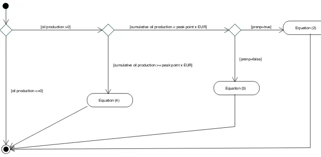
The behavioural rule4

for oil production is given in Figure 2 as an UML(Unified Modelling Language) activity diagram. ’Rounded rectangles’ represent the operations and the ’diamonds’ represent the decision points of the agents. The key idea is that oil production of attends to

’peak’ when approximatelypda of theea has been extracted (see Campbell 1996 and 1997).

In particular, ifpat= 0 then the agent always exist with production = 0 andisP rodat is set

to false. Ifpat >0, the agent checks if thecat is less than the proportion ofea * pda. If this is

true, then the agent checks if it is a pre-peak net producer - it can cover its domestic demand given in (1). If it is a pre-peak net producer, then following operation is selected:

pat =pat−1+dat−1+wdat−1 (2)

4

2.2 Data 2 MODEL DESCRIPTION

[oil production >0]

Equation (4) [oil production <=0]

[cumulative oil production < peak point x EUR] [prenp=true] Equation (2)

Equation (3) [prenp=false] [cumulative oil production >= peak point x EUR]

Figure 2: Simplified behavioural rule for oil production

If the agent is not a pre-peak net producer (prenp=false), then (3) is selected:

pat=pat₋₁+dat₋₁ (3)

If the cumulative production iscat >=ea∗pda, then (4) is selected:

pat =pat₋₁−(pat₋₁∗(pat₋₁/yat)) (4)

Note that (4) assumes that the decline rate is dynamic rather than fixed at the time of peak. Equation (2) uses wdat. This is given by

wdat =nwdt−1/nppnpt−1+ ((pat−1−mpt−1)/mpt−1)∗(nwdt−1/nppnpt−1) (5)

where nwdt₋1 is the net world demand at timet₋1,nppnpt₋1is the total number of pre-peak net producers at at t−1, mpt₋1 is the mean production from the pre-peak net producers. Effectively, (5) assumes that agents with largerpat₋₁would be more able to increase production

to meet net world demand.

It is important to clarify here that Equations (2) and (3) are adjusted (where necessary) based upon a maximum production growth fromtto t+ 1. This maximum production growth can be different for each country as shown in section 3 and 4.

2.2

Data

The ACEGES energy database is a collation of different sources of data5

• Petroleum production: i) ’World Petroleum Assessment 2000’ of the United States

Geo-logical Survey (USGS), ii) the ’CIA World Factbook 2010’ (CIA), iii) ’Campbell, Heapes - An Atlas of oil and gas deplation, 2008’ (CAM), iv) ’DeGolyer, MacNaughton - 20th Century Petroleum Statisitics, 1994 edition’ (DeMac), v) ’API - Petroleum Facts and Figures, 1971’ (API) and vi) ’EIA’s International Energy Data, Analyses, and Forecasts’ (EIA)

• Petroleum consumption: ’EIA International Energy Annual 2006’ (IEA)

• Consumption growth rates: i) ’EIA International Energy Outlook 2002’ (IEO) and ii) ’IEA

World Energy Outlook 2009’ (WEO)

5

2.2 Data 2 MODEL DESCRIPTION

The model outlined above is initialised as follows:

• Campbell and Heapes EUR: Data available for 62 countries. World total 1.9 trillion

barrels;

• CIA EUR: Data available for 93 countries. World total 2.4 trillion barrels;

• USGS EUR: the 5% estimate from USGS of the EUR. Data available for 53 countries.

World total 6.8 trillion barrels;

• Oil production in 2001;

• Oil cumulative production in 2001; • Oil consumption in 2001;

• IEO low growth rate : the lower estimate of the consumption growth rate according to

IEO;

• IEO high growth rate : the higher estimate of the consumption growth rate according to

IEO;

• WEO growth rate: the estimate of the consumption growth rate according to WEO.

2.2.1 Data Issues: Petroleum production

Data for production were reported at different dimensions: barrels, thousand barrels, million barrels and billion barrels. In ACEGES, the data is reported in million barrels per year. The ACEGES database contains oil production data from 1859 to 2008:

• From 1859 to 1964 data comes from API • From 1964 to 1994 data comes from DeMac • From 1994 to 2008 data comes from EIA

2.2.2 Data Issues: Variables construction

In order to construct some of the ’variables’ used by the ACEGES model, datasets from different sources were compiled:

• CIA EUR: CIA provides estimates of theproved reserves of oil at the beginning of 2009.

Therefore, the CIA EUR is the sum of i) the cumulative production for all the countries up to 2008 (using the data sources discussed above) and ii)proved reserves. Note that the CIA EUR does not include ’oil yet to discover’. The main advantage of the CIA EUR is the construction of EUR for 93 countries (through the collation of datasets from different data providers). This is important fornwdt₋1 used in Equation (5).

• Cumulative oil production in 2001: The country production up to 2001 using the data

sources discussed above.

2.2.3 Data Issues: Single country issues

Because ACEGES models 93 countries, most of the problems in modelling some of the 93 countries come from the difficulty in estimating the yearly and cumulative production of the ’breakup’ countries (e.g., Former Soviet Union). Country-specific data is not available to the ACEGES team for these countries for the period before the splitting.

3 GRAPHICAL USER INTERFACE OF ACEGES

was available after the splitting year. Then this share was used to estimate the cumulative production of country up to the splitting year.

Al thought this is a simplified way to estimate oil production for selected countries that can result in under- or over-estimation of country’s resources, the global production profile is not affected as most of the countries involved have a small share of the oil market (the exception is Russia where our estimates are very close to the estimates reported in the literature).

Specifically:

• Brunei and Malaysia: The majority of the production up to 1979 has been allocated to

Malaysia (60%).

• Czech Republic and Slovakia: The majority of production up to 1992 has been allocated

to Czech Republic (70%).

• Former Soviet Union6: Production up to 1992 has been allocated mostly to Russia (90%).

The remaining production was proportionally divided among the remaining oil producing countries of the FSU.

• Former Yugoslavia (Serbia and Croatia): The whole of the production up to 1991 has been

allocated to Croatia (65%) and Serbia (35%). The production of Serbia also includes Montenegro, while the small share of Slovenia (1%) has been allocated to Serbia and Croatia according to their shares.

• Neutral Zone (Saudi Arabia and Kuwait): Oil reserves in the Neutral Zone has been

assigned to the Saudi Arabia (50%) and to the Kuwait (50%).

3

Graphical User Interface of ACEGES

Since ACEGES uses the MASON Simulation Toolkit, the Graphical User Interface (GUI) of the ACEGES is based on MASON’s GUI.

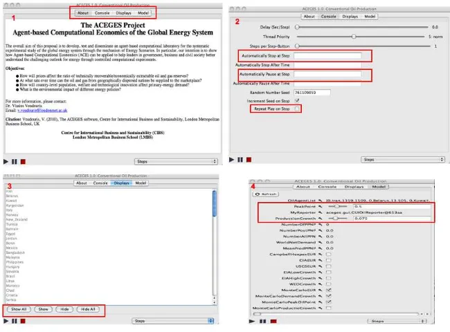
Once the ACEGES runs (by clinking on the ’ACEGES1.0.jar’ file), two windows will appear. One has the title bar labelled ’World Oil Production - All Countries’, and it is a display window. The other one is has the title bar labelled ’ACEGES 1.0: Conventional Oil Production’, and this is a console window. How to use the ’display window’ is explained in section 4. This section discusses the ’console window’ shown in Figure 3.

Figure 3-1 shows theAbout tabular panel. TheAbout panel shows some information about the ACEGES project whose main output is the ACEGES software.

TheConsole panel (Figure 3-2) contains useful settings for the simulation. The first three slides allow one to insert some delay time between each time step (in case the simulation is too fast), to increase the priority of the simulation thread, and to execute any number of steps upon pressing the play button (when the simulation is paused).Next, there are three text areas where one can specify the time step where the simulation shouldstoporpause(once stopped, a simulation cannot be resumed), or set therandom seed for the simulation to a certain value. By default, the random seed is incremented whenever the simulation is stopped (so that the next time the simulation is played, it runs with a different seed). Setting the last check button,Repeat Play on Stop, sets ACEGES to automatically start a new simulation whenever the old one is stopped. This is mostly helpful for kiosk modes and/or for the generation of a large number of Monte Carlo experiments (discussed in section 4) that can be analysed using a statistical package such as R (see also Figure 1 and Figure 13).

TheDisplay (Figure 3-3) panel allows one to select which displays will be shown, and which will not. Each display is identified by a unique name. To hide a display, the user needs to select

6

3 GRAPHICAL USER INTERFACE OF ACEGES

Figure 3: ACEGES Graphical User Interface

it in the list of displays, and then press theHide button. Alternatively, clicking on the display’s close button will hide it. To show a display, the user needs to select it in the list of displays, and then press theShow button. The user may show/hide all displays by pressing theShow all / Hide all buttons.

The last panel is theModel panel (Figure 3-4) - this panel is used to set the parameters of the simulated scenario. Note the Model panel allows the user to modify the parameters affecting the entire simulation and/or the parameters affecting a single agent (country). In the current implementation, users can rundiscretescenarios based upon specific values for the peak/decline point, EUR, oil demand growth and oil production growth. Users can also run continuous

scenarios7

by selecting one or more of the Monte Carlo boxes. For example, if a user wants to run a scenario that uses specific values for the peak/decline point, oil demand growth and oil production growth but not for the EUR, then the MonteCarloEUR box needs to be selected. Note that in this case the peak/decline and oil production growth is homogeneous for all the countries. Heterogeneity (each country can have a different peak/decline point and production growth) is introduced when the MonteCarloPeakOilPoint and MonteCarloProductionGrowth

boxes are selected.

Currently, the Monte Carlo experiments are based on the Uniform DistributionU(a, b). For (see also section 2):

• MonteCarloEUR:ais the minimum of the CIA, USGS and Champbell and Heapes

esti-mates andbis the maximum of the CIA, USGS and Champbell and Heapes estimates.

• MonteCarloDemandGrowth: ais the minimum of the EIA Low and WEO estimates and

bis the maximum of the EIA High and WEO estimates.

• MonteCarloPeakOilPoint: ais 0.35 andbis 0.65 (see Hallockat al, 2004). • MonteCarloProductionGrowth:ais 0.05 andbis 0.15 (see Hallockat al, 2004). 7

4 EXAMPLE: BUILDING ENERGY SCENARIOS

4

Example: Building energy scenarios

The ACEGES software can been seen as an user-centred (energy) scenario development tool. Once the software is started, the user sets the input variables using theModel tab. This example uses the Monte Carlo simulation (see Figure 4) for all of the four key variables discussed in section 2:

• EUR • Peak point

• Oil Demand growth • Oil Production growth

Figure 4: ACEGES: Model tab

By clicking on the ’pause’ button the simulated scenario starts. The simulated scenario can also be run step by step. In Figure 5 the specific scenario was stepped until step 18.

Clicking the ’pause’ button, the simulated scenario restarts automatically (as discussed in section 3 this is because the setting specified in theConsole tab). Using the ’pause’ button, the simulated scenario is stopped (note that here each step is one year and the first simulated year is 2002). By clicking on ’stop’ button, ACEGES ’re-initialises’ the simulated scenario (including the visualisations) using the settings of theModel panel (see Figure 6).

The results of the simulation can be visualized by selecting the country(ies) of interest from the Display tab. Figure 7 reports only one country to explain how to read and modify the graphical output (visualisation).

Figure 8 is the result of a Monte Carlo experiment for Saudi Arabia. The visualisation can be modified as desired. Figure 8 shows:

1. The EUR estimation selected by the Monte Carlo process.

4 EXAMPLE: BUILDING ENERGY SCENARIOS

3. The oil production growth selected by the Monte Carlo process.

4. The peak point selected by the Monte Carlo process.

5. The graph scale for oil production.

6. The graph scale for the Reserves/Production ratio.

Figure 5: ACEGES: Stepping the scenario

4 EXAMPLE: BUILDING ENERGY SCENARIOS

Figure 7: ACEGES Display

7. The graph scale for the Production /Cumulative Production ratio.

8. The line representing the series of oil production.

9. The line representing the evolution of the Reserves/Production ratio.

10. The line representing the evolution of the Production /Cumulative Production ratio.

11. The ’Save as PDF’ button: A way to save the chart as a PDF file. This can be done also right clicking on the graph.

Figure 9 is the World Oil Production (as discussed above, the world oil production is not modelled explicitly but is the emergent output of the decisions made by the individual countries). Figure 9 is very similar to Figure 8, but (1), (2), (3), (4), (7), (10) are not shown.

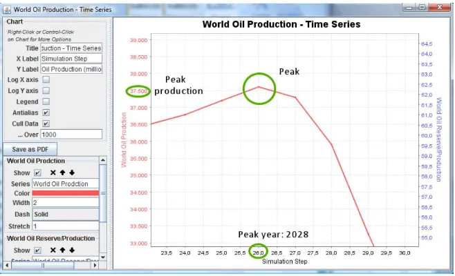
It is also possible to zoom the graph to observe what the behaviour of the series is in a certain interval or what the peak year and peak production is. There are two ways to zoom (see Figure 10):

1. Use the mouse:

• Left click at the left of the interval of interest • Hold the left button and select the area

• To go back to the full graph, left click in any point of the graph and move the mouse

in any direction

2. Use the options window:

4 EXAMPLE: BUILDING ENERGY SCENARIOS

Figure 8: Graphical output: Saudi Arabia

Figure 9: Graphical output: World Time Series

ACEGES also visualizes the evolution of the world production as a function of the contri-bution of each country (in different colours). The vertical distance by one color and the other represents the country production for each step (see Figure 11). The whole area covered by a single color represents a country’s cumulative production.

By zooming, contributors made by ’small’ player of the world oil production can be detected. By moving the mouse pointer, a tooltip shows: i) the name of country represented by the colour and ii) the world oil production up to the specified country (see Figure 12).

4 EXAMPLE: BUILDING ENERGY SCENARIOS

records the data for the world oil production. These files and then be analysed using a statistical software. For example, SimulatedOilData 1280661362016.csv was analysed using the R-based GAMLSS (see Rigby and Stasinopoulos, 2005) package and the results are shown in Figure 13.

Figure 10: World Production - Zooming

5 REFERENCES

Figure 12: World Oil Production - Zoomed market share of countries

Figure 13: Monte Carlo experiments for selected countries

5

References

Campbell C., (1996), ”The status of world oil depletion at the end of 1995”. Energy Exploration and Exploitation, 14(1), 63-81.

Campbell C., (1997), ”Depletion patterns show change due for production of conventional oil”. Oil and Gas Journal, 95(52), 33-7.

5 REFERENCES

Hallock, J.L., Tharakan, P., Hall, C.A.S., Jefferson, M., Wei, Wu., (2004), ”Forecasting the limits to the availability and diversity of global conventional oil supply”, Energy 29, 1673-1696.

Rigby, R. A. and Stasinopoulos D. M. (2005), ”Generalized Additive Models for Location, Scale and Shape, (with discussion)”, Appl. Statist., 54, pp 507-554.