Branching Process based Cascading Failure Probability Analysis for a Regional Power Grid in China with Utility Outage Data

Branching Process based Cascading Failure Probability

Analysis for a Regional Power Grid in China with Utility

Outage Data

Hui Ren1_{, Ji Xiong}1_{, David Watts}2,3_{, Yibo Zhao}4 1

Department of Electrical Engineering, North China Electric Power University, Baoding, China

2

Pontificia Universidad Catolica de Chile, PUC, Vicuna Mackena 4860, Macul, Santiago, Chile

3

University of Wisconsin-Madison, Wisconsin, USA

4

School of information & Electronic Engineering, Beijing Institute of Technology, Beijing Email: [email protected], [email protected]

Received April, 2013

ABSTRACT

Studying the propagation of cascading failures through the transmission network is key to asses and mitigate the risk faced the energy system. As complex systems the power grid failure is often studied using some probability distribu-tions. We apply 4 well-known probabilistic models, Poisson model, Power Law model, Generalized Poisson Branching process model and Borel-Tanner Branching process model, to a 14-year utility historical outage data from a regional power grid in China, computing probabilities of cascading line outages. For this data, the empirical distribution of the total number of line outages is well approximated by the initial line outages propagating according to a Borel-Tanner branching process. Also for this data, Power law model overestimates, while Generalized Possion branching process and Possion model underestimate, the probability of larger outages. Especially, the probability distribution generated by the Poisson model deviates heavily from the observed data, underestimating the probability of large events (total no. of outages over 5) by roughly a factor of 10-2 to 10-5. The observation is confirmed by a statistical test of model fitness. The results of this work indicate that further testing of Borel-Tanner branching process models of cascading failure is appropriate, and should be further discussed as it outperforms other more traditional models.

Keywords: Cascading Failure; Poisson; Power Law; Branching Process; Generalized Poisson; Borel-Tanner

1. Introduction

Cascading failure is the process by which initial outages of components of the electric power transmission system can occasionally propagate to more widespread outages and large blackouts. These blackouts involve complex chains of events, that are not completely independent, as an outage that have already occurred weakens the system, making the systems more vulnerable and further outages more likely [1].

Since 2001, researchers with multiple backgrounds of electrical engineering, mathematics, physics and nonlin-ear dynamics have work more heavily addressing this topic from different angles. This research on cascading models is surveyed and presented in [2,3], and is mainly focused on 1) studying on the evolution of cascading failure from a long term point of view; 2) studying on the effect of specific disturbances on cascading propagation; 3) identifying the vulnerable area of the system accord-ing to the topological features; 4) evaluataccord-ing hazards the initial failure could cause to the system by identifying the

afterwards cascades being initiated. All these researches provide helpful research results.

Dealing with these issues and performing risk assess-ment requires often identifying the probability distribu-tion of blackout size. It has been widely observed that the probability distributions produced by models in above-mentioned research works have approximate power law regions that cannot be produced by independent outages and are broadly consistent with the characteristics ob-served in the utility historical outage data from several countries.

the difficulties addressing complexity and non-inde- pendency among different events.

1.1. Probabilistic Models for Utility Outages

While the literature body in this field is very broad, this section summarizes previous work on probabilistic mod-els for utility outages that relates more closely to our work.

Chen and McCalley, after analyzing the North Ameri-can transmission line outaged data in [4], proposed an accelerated propagation model for the number of trans-mission line outages [5]. They try a generalized Poisson distribution and a negative binomial distribution for the accelerated propagation model. The fitness test of the accelerated propagation model to the reference utility outage data showed, for the PDF of the number of line outaged, the proposed exponentially accelerated cascad-ing model on the probability of outages with more than 6 lines fit better than other models (0.00061 for accelerated propagation model, while 0.00053 for the observed out-age data, probabilities produced by Generalized Poisson model and Negative Binomial model are one order of magnitude smaller that that of the observed data).

In [1], Ren and Dobson demonstrated a way to test a branching process based bulk statistical model of cas-cading line outages on industry data. The model de-scribed the development of cascading failure starting from initial outages that then propagates in stages. The average amount of propagation was estimated and hence the probability distribution of the size of the cascading failure (measured by the total number of line outages) was predicted. The fit of the model is examined with a 9-year historical outage data set from a regional power grid. Furthermore, Dobson [6] improves the branching process model in [1] by considering variant propagation in different stages, modeling the increases of propagation as the cascade proceed following the observation in the utility data [8]. The branching process model is then used to predict the distribution of total number of outages for a given number of initial outages. They study how the total number of lines outaged depends on the propagation as the cascade proceeds.

1.2. Proposed Research

The power system is carefully designed and operated so that most transmission line outages do not propagate over the system and it only has to encompass one or few out-ages occurring together. This paper deals exactly with those situations where failure may propagate, protections, controls and other factors may not operate as desired, and several components of the system may be affected. As previous references, failure propagation is modeled using probabilistic models, allowing for multiples failures

modes.

Power grids differ one from another mainly in topol-ogy, size, capacity, interconnectedness, loading level, and several other physical/technical features. The plan-ning and operation of the market or the power system also varies, but not as widely as physical features (dis-patch rules, unit commitments, market clearing processes differs but have similar goals and results).

Although these differences exist, outage data seems to suggest similar cascading failure behavior in widely dif-ferent systems. As such, research is still undergoing aiming to identify the best probabilistic models for cas-cading modeling in power systems. In this paper, we compare the fitness of 4 different statistical models to the 14-year utility outage data from a regional power grid.

This paper is organized as follows. In section II, out-age data sources and handling procedures to group fail-ures are presented. In section III three probabilistic mod-els ever used for transmission line outage analysis are introduced first. Utility outage data is introduced in sec-tion III, and also the simple grouping techniques of util-ity outage data for branching process based analysis.

2. Utility Outage Data

Cascading failure models are very constrained by outage data availability and some models require some pre- possessing or handling the data. This section address these topics, describing different data sources, the data set used here and the handling procedures required to fit the models.

2.1. Main Sources of Utility Outage Data

For the researches on cascading large blackouts, the util-ity outage data are valuable references on modeling and useful diagnostics in monitoring the process and extent of blackouts. Since data is scarce, here we summarize the data available from cited references.

Ref. [4] summarized the results of a survey of design characteristics of and outage experience with overhead transmission at voltage 230kV and above in USA and Canada, for a purpose of providing technical support on the probabilistic system models for planning and opera-tion. The outage data were submitted by utilities from all nine NERC/USA reliability regions and by the Canadian Electric Association representing all of Canada. The sta-tistics provided classifications and analysis on 38,489 outage data according to voltage level, region, causes, or duration time, etc.

Ref. [8] provides a historical outaged data recorded by a North American utility over a period of 12.4 years and is being upgraded constantly. The transmission line out-age data is required by NERC for the Transmission Availability Data System (TADS). The data for each transmission line outage includes the outage time (to the nearest minute) as well as other data. All the line outages are automatic trips. More than 99% of the outages are of lines rated 69kV or above and 97% of the outages are of lines rated 115kV or above. There are several types of line outages in the data and a variety of reasons for the outages [6].

Our previous research and the work of this paper are based on 9-year historical outage data in [1] and 14-year outage data in this paper, which are extracted from the fault data information recorded by protective relays in a regional power grid. The data we can reach provides the voltage level and the time stamp of the failure, the se-quence of the failures, and failure cause, however with on specific information on load shed. The data set is de-scribed in details in next section.

2.2. Utility Outage Data Used in this Paper

The outage data used in this paper is from a regional electric power transmission system with, approximately, 190 220kV buses, and 12 buses at 500kV. The data is recorded over about 14 years staring in 1997 and ending in 2011.

The historical outage data is extracted from the report containing the outage details recorded by fault recorder devices and the fault analysis by relay engineers. The extracted information includes the contingency type (transmission line failure, or busbar failure, or generator failure…), contingency time (to the nearest minute), vol-tage level, and the auto-recloser’s action. In this research, only transmission line outages in 220kV and 500kV are computed in the model. Outages at lower voltage levels are not considered because of the potential number of unrecorded events.

When processing the outage data, the voltage level, line outage type (single phase or three-phase and detailed causes of the line outages are neglected, and are regarded as the same. The neglecting in the bulk statistical analy-sis is appropriate, for no matter what the details on caus-es, type or voltage levels are, and they all result in the weakness of the transmission system to various extent. The more sever the outage is (outages on higher voltage level, or more initial outages, or poor operation and con-trol techniques), the more sever outcomes follows, such as even more outages, while bulk statistical analysis based on the historical outage data actually takes all of these into consideration, and lead to a more credible evaluation on system’s risk level.

Large flashover events in the data with approximately 260 outages over two days are neglected because of lacking time tags. There is not large cascading blackout (totally blackout) in this regional power grid over the analyzed horizon. Data recording is not perfect and there is some kind of incomplete outage data recording, those should be smaller failures, not big ones. Therefore the tail part in the probability distribution (PDF) versus out-ages with various sizes should be credible.

[image:3.595.308.540.570.717.2]

The clustering of outages in stages can be seen in

Figure 1. The x-axis shows time since start of cascade for outages in each of the 458 cascades. The first min of each cascade is shown. Multiple outages at the same time are shown slightly displaced.

2.3. Data Grouping by Stages

The processing in this section for the outage data is mainly for the application of branching process model. Here, we follow the data grouping technique in [1]. The outage data are grouped according to their time stamps without considering the geographical information of the outage. Although successive outages in areas far way from each other may not have direct electrical connec-tions, but the successive happening does suggest a further weakening of the system. Moreover, when the data is in bulk and the system is in large-scale, the difficulty from considering more detail information of each outage would compromise the application of the method.

Successive outages separated in time by more than one hour are assumed belong to different cascades, for op-erator actions are usually completed within one hour. Successive outages in a given cascade separated in time by more than one minute are assumed in different stages within that cascade, for transients or auto-recloser actions are completed within one minute.

733 outages are abstracted from the failure records, and from them, 459 cascades are obtained by the intro-duced grouping technique. Table 1 is obtained by sum-ming over all the 459 cascades the number of outages in

[image:4.595.55.288.292.375.2]

each stage. That is, of the 733 outages, 556 are in stage 0 of a cascade (for some cascades, there are more than 1 failures in stage 0), 83 are in stage 1 of a cascade, and so on. Failures in stage 0 are defined belong to initial failure of a cascade in the following analysis.

Table 2 and Table 3 give the statistics of the no. of lines lost in each initial failure, and in each cascade, re-spectively. N-r in Tables 2 and 3 means the loss of r transmission lines in the power system (a traditional re-liability event indicator). The number of line outages in initial failures could be as large as 7, and the total num-ber of outage in the cascade is at most 19, however the probability of these severe occasions are extremely small.

Table 1. Number of outages in each stage summed over the cascades.

Stage Failure _No. Stage Failure _No. Stage Failure _No. Stage Failure_No.

[image:4.595.56.288.414.530.2]

Z0 556 Z4 14 Z8 3 Z12 2 Z1 83 Z5 6 Z9 3 Z13 1 Z2 31 Z6 5 Z10 3 Z14 1 Z3 20 Z7 3 Z11 2 Z15 0 Table 2. Statistics on the no. of transmission line lost in the initial failure.

Con. Type of initial failure No. Probability

N-1 402 0.8758

N-2 35 0.07625

N-3 13 0.02832

N-4 5 0.01089

N-5 0 0

N-6 3 0.006536

[image:4.595.312.537.531.709.2]

N-7 1 0.002179

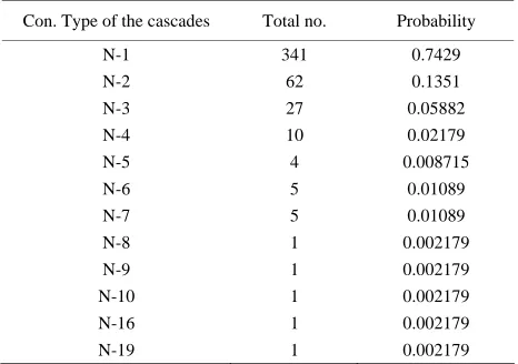
Table 3. Statistics on the total no. of transmission line lost in a cascade.

Con. Type of the cascades Total no. Probability

N-1 341 0.7429

N-2 62 0.1351

N-3 27 0.05882

N-4 10 0.02179

N-5 4 0.008715

N-6 5 0.01089

N-7 5 0.01089

N-8 1 0.002179

N-9 1 0.002179

N-10 1 0.002179

N-16 1 0.002179

N-19 1 0.002179

The probability distribution (PDF) of initial and total line outages are shown in Figure 2 on a log-log scale. Raw data is shown in Figure 2 with no binning. It has a peak at 6 and 7 outages. One reason for this is that some cascades are initiated by a bus outage, and the relay trips off all transmission lines connected to that bus simulta-neously at the start of the cascade. On log-log scale, the PDF is roughly a straight line, showing a “heavy tail”, consistent with researches on cascading blackouts in [10].

3. Assessing Four Probabilistic Models

We introduce in this section four different probability models which we use to estimate the distribution of the total number of line outages in this paper. Among these models, branching process model is introduced as a focal point and will be compared with other traditional prob-ability models using fitness test.

3.1. Traditional Poisson Model [9]

Consider a random variable T{0,1}, with T 1 rep-resenting the event of an individual line tripping and the probability is P T(  1) p. Then the probability of tripping of each line can be represented as

1

( | ) t(1 ) t, 0,1; 0

P T t p p p  t  p 1 (1) Suppose that the total number of lines in a power sys-tem is N, and each line has the same probability p to be tripped and each trip event is independent of any other one. Then the probability distribution of total number of line outages Z subjects to the binomial distribution:

[ ] r r(1 )N r, 0,1, 2, ,

N

P Zr C p p  r  N (2) Consider that N is large and p is small under general conditions, then the formula can be approximated by the Poisson distribution with a parameter of conNp:

[ ] (1 )

con / !, 0,1, 2, ,

r r N r N

r con

P Z r C p p

e   r r





  

   N (3)

[image:4.595.56.289.569.733.2]

In this paper, we use maximum likelihood estimation [15] to estimate the parameter con. If the space X is

discrete with probability distributi unction

( ) ( ; )

P X x p x

on f



  ,

then the joint probability distribution function of event

1 1 2 2

{X x X, x,,X_nx_n} can be shown as

n

1

1

( ) ( , , _n; ) ( ; )

i

L L x x  p x_i 



  



(4)

where  ter

is the model parameter to be estimated. The parame value 



which makes (4) reach the maxi-mum value is called as maximaxi-mum likelihood estimator, we can find out 



by mathematical methods such as derivation.

We can get based on Table 2 and m

(5)

3.2. Power Law Model [10-11]

a normalized

dis-6)

When we draw the relationship of on

power law

(7)

3.3. Branching Process Model [1]

0.5970

con

 

ood estimatio



aximum likelih n. The estimated distribu-tion is as follows:

 

  0.5970 1

[ ] 0.5970r / ( 1)!, 1, 2,

P Z r e r r 

The total number of line outages Z has

tribution as shown in (6) when it follows a power law:

[ | ] q/ q, 0; 1, 2,

P Zr q r



r q r  (

[ ]

P Zr

t line wi and r

a log-log plot, we will find a straigh th slop

/ q

q r





, this indicates the distribution follows a . Using maximum likelihood estimation

intro-e

duced above, we can get q 2.0



 based on Table 2, then the expression of using po aw model to estimate the distribution of outage lines can be shown as follows:



  

wer l

2.0 2.0 2.0

1

[ ] / 0.645 , 1, 2,

k

P Z r r r r r



 



  

The propagation  which means the mean number of child failures for each parent failure plays a critical role in branching process. We consider  as an invariant constant in this paper, the positive nu ber of failures in stage zero 0

m

Z will produce outages in the next stage with a mean number of Z0, the child failures then

be-come parents to produce ges with a mean number of

2 0

outa

Z

 in the next stage and so on [12]. Here we use the d introduced in [1] to estimate

metho :

( ) ( ) ( )

1 2 ( )

1

( ) ( ) ( )

0 1 ( ) 1

1 ( ( ) ) N i i J

i i i N i i

Z Z Z

Z Z Z

          





  (8) where J

i i i

represents the total number of line outages,

p ( )

N i re resents the maximum stage with nonzero fail-Based on Table 1 and (8), we can know

ures.

J

1 2 14

0 1 13

0.24

Z Z Z

 _{  }

Z Z Z

  

   (9)

1. Generalized Poisson model

numbers follows a

3.2.

If the distribution of initial failure

Poisson distribution with the parameter  and ignores the condition with zero initial failure, the istribution of initial numbers is as follows:

d

0

[ ] , 1, 2,

(1 ) !

r

e

P Z r r

e r

  

  (10)

e mean number of initial failures can be shown Th

0 / (1 )

Z  e 



 

  (11)

n get

We ca Z0 1.211 base

ator

d on Table 2, and then we get the estim .3965 using (11). The distri-bution of the total num outages under this con-dition follows generalized Poisson distribution [13] as shown in (12).

ˆ ₀

 

ber of line

1

0.24 0.3965 1

0.3965

[ ] ( )

(1 ) !

0.3965(0.24 0.3965) ,

(1 ) !

3.2.2. B 1, 2 r r r r e

P Z r r

e r e r e r r                        (12) orel-Tanner model

ollows arbitrary distribution, If the initial failure numbers f

then the total number of line outages follows a Borel- Tanner distribution [14].





0

0

0 0

1

1 0 0 0

0

0.24 1

1 0 0 0

0

0

( )

( )

0.24 (0.24 )

( )!

1, 2, ; 1, 2,

r r z r z r r z r z e !

r P Z z z r

r z

e

P Z z z r

r z

r z r

              _  _       _     (13) P Z  

where P Z 0 z0 Table 2.

can be calculated based on the data

4. Comparison Analysis of 4 Probabilistic

he expressions in (5), (7), (12), and (13) for given in

Models

evaluate t We

the loss of different number of lines, i.e.



1, 2, 3, 4, 5,...,10



r .

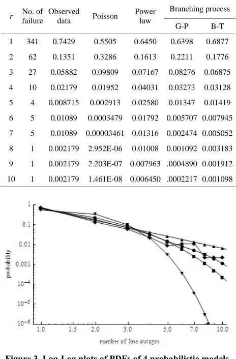
probabilities in Table 4 are given in Figrue 3. Figrue 3 shows Log-Log plots of PDFs in Poission model in (5) (Inverse triangles), Power Law model in (7) (triangles), Generalized Poisson branching process in (12) (squares), Borel-Tanner branching process in (13) (diamonds) and observed data (dots).

For outages fewer than 5, all models fit well (as shown in

view, the probability dis-tri

able 4. Probabilities from 4 Probabilistic Models and

[image:6.595.312.534.81.248.2]

Ob-Branching process Figure 3). However, Borel-Tanner branching process model is better than the other 3 models for outages big-ger than losing 5 lines. Power law overestimates the probability of larger outages. The curve generated by the Poisson model deviates heavily from the observed data, underestimating the probability of large events (r>5) by roughly a factor of 10-2 to 10-5.

In order to get a more clear

bution of total number of outages from observed data and estimated using Borel-Tanner branching process are given in Figure 4. We can see that the distribution esti-mated using Borel-Tanner branching process can fit the distribution from data well, and in the log-log plot it also shows a heavy tail.

T

served Data.

r No. of Observed Poisson Power failure data law

[image:6.595.56.288.377.730.2]

G-P B-T 1 341 0.7429 0.5505 0.6450 0.6398 0.6877 2 62 0.1351 0.3286 0.1613 0.2211 0.1776 3 27 0.05882 0.09809 0.07167 0.08276 0.06875 4 10 0.02179 0.01952 0.04031 0.03273 0.03128 5 4 0.008715 0.002913 0.02580 0.01347 0.01419 6 5 0.01089 0.0003479 0.01792 0.005707 0.007945 7 5 0.01089 0.00003461 0.01316 0.002474 0.005052 8 1 0.002179 2.952E-06 0.01008 0.001092 0.003183 9 1 0.002179 2.203E-07 0.007963 .0004890 0.001912 10 1 0.002179 1.461E-08 0.006450 .0002217 0.001098

Figure 4. PDFs of total No. of outages from observed data

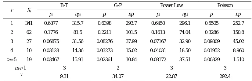
Chi-square test is then used to provide a quantitative co

(dots) and by Borel-Tanner branching process (line).

mparison among 4 models, and the test result is given in Table V. The Chi-square test [21] is widely used in statistics to test the fitness of a probability model to sam-ple data. Suppose X follows the discrete distribution with the possible values of 1, 2,,k, and the probability can be shown as P X(  i) p_i,1 i k. If we perform

n trials, and the event X i results X i_i( 1, 2,, )k

es, then we can use tatistic

tim the s 2 to show how much the samples deviate from the ribution to be tested:

dist

2 2

1

( )

k

i i

i i

X np np











(14)

when n , 2

follows the chi-square distribution

2

 w f om number k1. We can obtain (14) that the larger the statis 2

ith the reed

from tic  , the larger the deviation. Since the condition to let conclusion in-troduced above be true is that the distribution must be a polynomial distribution and all of the npi should be

larger than 5, we decompose the sample space into 5 ex-clusive sets

the

1 2 3

4 5

{1}, {2}, {3}, {4}, {5, 6, }.

M M M

M M

  

  

s

The test result is shown in Table 5. If there are es-timated parameters in the probability model, the freedom number of the 2 distribution should be changed to

1

k s . For instance, for the Borel-Tanner model,  meter to be estimated, so the freedom number chi-square distribution is 5-1-1=3; but for the generalized Poisson model, the parameters that should be estimated are

is a para of

 and , so the freedom number is changed to be 5-2-1=2. By i specting n Table 4, the value of 2 calcu-lated from the Borel-Tanner model is obvious smaller than the values gotten from other models, that illustrates the Borel-Tanner model is far more fit than the other

ly

[image:6.595.57.287.377.718.2]

st Results For all models.

[image:7.595.89.502.100.234.2]

B-T aw Poisson

Table 5. χ2 _Te

G-P Power L

r Xi

pi npi pi npi pi npi pi npi

1 341 0.6877 315.7 6390. 8 293.7 0.6450 296.1 0.5505 252.7 2 62 0.1776 81.5 0.2211 101.5 0.1613 74.04 0.3286 150.8 3 27 0.06875 31.56 0.08276 37.99 0.07167 32.90 0.09809 45.02 4 10 0.03128 14.36 0.03273 15.02 0.04031 18.50 0.01952 8.960 >=

r-1 3 2 3 3

9. 3 2 2

5 19 0.03467 15.91 0.02361 10.84 0.08172 37.51 0.00329 1.510

m

-χ2 _{31 4.07 2.87 92.4}

odels. When we set the significance level be 0.01, m

the2 of the Borel-Tanner model satisfies

2 2

(3) 11.34

 0.01  ,

that illustrates the Borel- Tanner model can exactly

de-5. Conclusions

ilistic models, Poisson model, Power scribe the distribution of real data under a significance level of 0.01.

We apply 4 probab

Law model, Generalized Poisson Branching process model and Borel-Tanner Branching process model, to a 14-year historical outage data from a regional power grid in China, computing probabilities of cascading line out-ages. We group the line outages into cascades and stages according to their outage times. For this data, the em-pirical distribution of the total number of line outages is well approximated by the initial line outages propagating

 according to a Borel-Tanner branching process with opagation parameter. For this data, Power law model overestimates the probability of larger outages, while the probability distribution generated by the Poisson model deviates heavily from the observed data, underestimating the probability of large events (outage no. greater than 5) by roughly a factor of 10-2 to 10-5. The observation is confirmed by a statistical test of model fitness. The re-sults of this work justify further testing of Borel-Tanner branching process models, leading to a promising re-search avenue for cascading failure modeling.

pr

6. Acknowledgements

ted from National Science

REFERENCES

[1] H. Ren and I. ission Line Outage

Data to Estimate Cascading Failure Propagation in an Electric Power System,” IEEE Transactions on Circuits and Systems, Vol. 55, No. 9, 2008, pp. 927-931.

doi:10.1109/TCSII.2008.924365

[2] IEEE PES CAMS Task Force on understanding, pred tion, mitigation and restoration of

cascading failures,

Ini-s for CaIni-scading Failure AnalyIni-siIni-s in TranIni-smiIni-sIni-sion

anadian Over-tial review of methods for cascading failure analysis in electric power transmission systems,” IEEE Power Engi-neering Soc. General Meeting, Pittsburgh PA USA, Jun. 2008.

[3] D. Watts and H. Ren, “Classification and Discussion on Method

System,” ICSET, Singapore, Nov. 2008.

[4] R. Adler, S. Daniel, C. Heising, M. Lauby, R. Ludorf and T. White, “An IEEE Survey of US and C

head Transmission Outages at 230 kV and above,” IEEE Transactions on Power Delivery, Vol. 9, No. 1, 1994, pp. 21 -39.doi:10.1109/61.277677

[5] Q. Chen, C. Jiang, W. Qiu and J. D. McCalley, “Probabil-ity Models for Estimating the Probabilities of Cascading Outages in High-voltage Transmission Network,” IEEE Transactions on Power Systems, Vol. 21, No.3, August 2006, pp.1423-1431. doi:10.1109/TPWRS.2006.879249 [6] I. Dobson, “Estimating the Propagation and Extent of

Cascading Line Outages from Utility Data with a Branch-ing Process,” IEEE Transactions on Power Systems, Vol. 27, No.4, 2012, pp. 2146-2155.

doi:10.1109/TPWRS.2012.2190112

[7] Information on Electric System D America can be Downloaded from th

isturbances in North e NERC Website at

for Self-organized Criticality in Electric http://www.nerc.com/dawg/database.html.

[8] Bonneville Power Administration Transmission Services Operations & Reliability website

http://transmission.bpa.gov/Business/Operations/Outages. [9] Q. Chen and J. D. McCalley, “A Cluster Distribution as a Model for Estimating High-order Event Probabilities in

Hui Ren thanks the suppor

Research Foundation of China (51107040), and thanks engineers from the regional power grid for the providing of the historical outage data for research. David Watts thanks the supported from Fondecyt project 1110527.

Power Systems,” 8th International Conference on Prob-abilistic Methods Applied to Power Systems. Ames, Iowa, 2004, 622-628.

[10] B. A. Carreras, D. E. Newman, I. Dobson and A. Poole, “Initial Evidence

Power System Blackouts,” Proceedings of the 33rd An-nual Hawaii International Conference on System Sci-ences, 2000, pp. 1411-1416.

doi:10.1109/HICSS.2000.926768

[11] I. Dobson, J. Chen, J. Thorp, B. A. Carreras and D. lackouts in Power

E. Newman, “Examining Criticality of B

System Models with Cascading Events,” Proceedings of the 35th Annual Hawaii International Conference on System Sciences, 2002, pp. 803-812.

doi:10.1109/HICSS.2002.993975

[12] I. Dobson, B. A. Carreras and D. E. Ne ing Process Approximation to Cascading

wman, “A B Load-dependen

as, V. E. Lynch

. Lynch and D.

ics for Engineers &

ranch-t

Scientists, Seventh Edition. Pearson Education Asia Lim-ited and Tsinghua University Press.

System Failure,” The 37th HICSS. 2004.

[13] I. Dobson, K. R. Wierzbicki, B. A. Carrer

and D. E. Newman, “An Estimator of Propagation of Cas-cading Failure,” the 39th HICSS．2006．

[14] I. Dobson, K. Wierzbicki, B. A. Carreras, V

E. Newman, “An Estimator of Propagation of Cascading Failure,” The 39th HICSS, 2006.