Wireless Background Noise in the Wi-Fi Spectrum
Bo Fu, Gábor Bernáth, Ben Steichen, Stefan Weber
Department of Computer Science and Statistics,Trinity College Dublin, Ireland
E-mail: {bofu, bernathg, ben.steichen, stefan.weber}@tcd.ie
Abstract—Background noise constitutes an often-neglected factor
in the investigation of solutions for wireless networks. Experiments carried out in these networks tend to ignore the presence of background noise and primitive noise simulators are used to create environments that resemble real-world characteristics. While such assumptions and experimental setups create perfect world scenarios that allow a normalized evaluation of solutions, they fail to capture transmission characteristics as they are experienced in the real world. This paper concentrates on the investigation of background noise in wireless networks, presenting a large amount of data determining a diversity of wireless noise levels that are collected over a twenty-four hour period on a busy university campus, and highlighting the importance of accounting wireless noise when experimenting in the Wi-Fi spectrum.
Keywords- wireless background noise; wireless networks; network measurement
I. INTRODUCTION
Over the last decades, wireless communications have become an essential part of our daily life. Not only research and universities but also businesses and enterprises are hugely dependent upon wireless technologies. As the number of wireless networks increases, the environment that these networks share becomes increasingly saturated with signals from a variety of sources. As a result, an increasing number of transmissions interact and interfere with one another and cause unforeseen problems for communication protocols.
In the development of communication protocols, the presence of other sources of transmissions is generally regarded as a source of errors. The evaluation of these protocols, however, focuses on the demonstration of the exploitation of available bandwidth, the optimization of access to the medium and the provision of functionality. These evaluations are generally carried out in simulators that provide little or no representation of additional sources of transmissions that would interfere with the performance of a protocol. The examination of the behaviour of protocols in the presence of increasing background noise has largely been neglected and leads to poor performance of existing protocols in real-world scenarios. This paper presents measurements of wireless background noise recorded on a busy university campus over a twenty-four hour period, showing how wireless noise varies throughout the day and suggests several implications for future research in the area of measuring background noise in wireless networks. Section II discusses possible causes of wireless background
noise and reviews related work in the research area. Section III details the setup of the experiments and their executions; findings from the experiments are then presented and analysed in section IV. Finally, section V concludes with suggestions of possible future research directions in the area of measuring background noise in wireless networks.
II. BACKGROUND
A. Possible Causes of Wireless Background Noise
Many sources can be a cause of background noise in a wireless network, for example, signals originating in an unlicensed frequency band may interfere with the intended frequencies of a network. Since the 2.4 GHz band used by 802.11b and 802.11g includes frequencies that are used by many different types of devices such as radios, microwave ovens, cordless telephones and Bluetooth devices etc, noise can be transmitted either accidentally or deliberately. Also, unwanted signals coming from distanced channels may act as noise for a given wireless network. Furthermore, noise may be generated by wireless networks themselves if their signals are corrupted by the environment and become unusable. A common cause of this is multi-path reception, where a signal reaches the receiver by different routes, i.e., if it is reflected off a concrete wall, and interferes with itself.
B. Related Work
flooding protocol using the random waypoint model and find that the results reported by the simulators vary greatly. The propagation models by simulators are too simple and that each of the simulators uses a different abstraction. The authors conclude that the differences of the results stem from the implementations of the simulators and that the incorporation of realistic environmental parameters would make the simulation too complex.
Kurkowski et al. [9] compare a large number of evaluations that have been reported in publications over the course of five years in major conference on ad hoc networks, MobiHoc. They conclude that most simulations use their own, very specific parameters that prevent the direct comparison of simulation results. Background noise was not a parameter that was considered in the comparison of the simulations.
Lee et al. [10] investigated the impact of noise modeling on the communication in wireless sensor networks. They measured the noise level in the 2.4 GHz band with regards to 802.15.4 in a number of locations such as the Grand Canyon, a library building and the Great Salt Desert. The traces from these measurements were used to evaluate packet delivery ratios in a variety of sensor network simulators.
Su et al. [11] aim to model background noise for simulators. They measured the noise level of eight routers on a floor of an office building during a sixteen-hour period and used these measurements as the basis for an analytical model. This model was then incorporated in the simulator Glomosim.
III. EXPERIMENTAL SETUP
A. Hardware and Software
Five Fujutsu Siemens Lifebook B Series notebooks with identical configuration were used as measurement nodes. All the notebooks were running a Linux operating system and an identical configuration was achieved by duplicating disk drives. Also, the clocks of these notebooks were synchronized before the execution of the experiments. The drift of the clocks during the experiments was negligible.
The Metageek Wi-Spy 2.4 GHz spectrum analyser [12] was used to capture the background noise in the 802.11b/g radio frequency band. The Wi-Spy analyser is capable of measuring noise amplitude for 86 frequencies (2400 – 2485 MHz) at a rate of 20 Hz. The amplitude is represented as an integer in the range of -97 dBm and -50.5 dBm. The experiments employed the open-source Wi-Spy-Tools software bundle [13] to record the raw data in CSV format. In addition, the measurement nodes were equipped with Cisco Aironet 350 PCMCIA wireless cards [14] with two omni-directional antennas connected. Since an active sniffer such as NetStumbler transmits packets to associate with access points, as a result, it would interfere with measurements recorded by Wi-Spy analyser. Therefore, a passive sniffer was used in the experiments, namely Kismet layer 2 wireless sniffer [15]. This sniffer provided the recording of advertised networks along with access points and was configured to channel hopping at a frequency of 1 Hz.
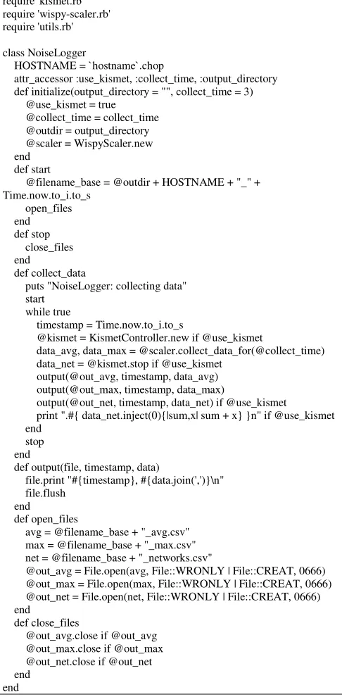
The measurement nodes were running a script written in Ruby programming language [16] to enable fast prototyping and experimenting. The script controls the wispy_logger and the kismet_server processes, while the later pre-processes the outputs generated from the wispy_logger that includes downscaling, time-stamping and final logging of the data. It also takes care of channel hopping when Kismet fails to channel hop using the Cisco Aironet network interface controllers. The kismet_server instance was terminated after three minutes to extract logfiles containing the number of wireless networks detected as well as the channels they were transmitting on. Figure 1 shows the code snippet of the noise-logger ruby script, and wispy-scaler.rb is shown in figure 2.
require 'kismet.rb' require 'wispy-scaler.rb' require 'utils.rb'
class NoiseLogger
HOSTNAME = `hostname`.chop
attr_accessor :use_kismet, :collect_time, :output_directory def initialize(output_directory = "", collect_time = 3) @use_kismet = true
@collect_time = collect_time @outdir = output_directory @scaler = WispyScaler.new end
def start
@filename_base = @outdir + HOSTNAME + "_" + Time.now.to_i.to_s
open_files end def stop close_files end
def collect_data
puts "NoiseLogger: collecting data" start
while true
timestamp = Time.now.to_i.to_s
@kismet = KismetController.new if @use_kismet
data_avg, data_max = @scaler.collect_data_for(@collect_time) data_net = @kismet.stop if @use_kismet
output(@out_avg, timestamp, data_avg) output(@out_max, timestamp, data_max)
output(@out_net, timestamp, data_net) if @use_kismet
print ".#{ data_net.inject(0){|sum,x| sum + x} }n" if @use_kismet end
stop end
def output(file, timestamp, data)
file.print "#{timestamp}, #{data.join(',')}\n" file.flush
end def open_files
avg = @filename_base + "_avg.csv" max = @filename_base + "_max.csv" net = @filename_base + "_networks.csv"
@out_avg = File.open(avg, File::WRONLY | File::CREAT, 0666) @out_max = File.open(max, File::WRONLY | File::CREAT, 0666) @out_net = File.open(net, File::WRONLY | File::CREAT, 0666) end
def close_files
@out_avg.close if @out_avg @out_max.close if @out_max @out_net.close if @out_net end
[image:2.595.312.555.212.707.2]end
require 'wispy-controller.rb' require 'utils.rb'
class WispyScaler
@@VALUE_COUNT = 86 def initialize
@wispy = WispyController.new end
def collect_data_for(timeout) data_count = 0
data_sum = [0] * @@VALUE_COUNT data_max = [-1000] * @@VALUE_COUNT while_timeout(timeout) {
line = @wispy.get_wispy_line data_sum.each_index { |i| data_sum[i] += line[i]
data_max[i] = line[i] if line[i] > data_max[i] }
data_count += 1 }
puts "WispyScaler: collected #{data_count} datasets" if $DEBUG raise "WispyScaler: No WiSpy data collected" if data_count == 0 data_avg = data_sum.map { |sum| (sum / data_count.to_f).round } [data_avg, data_max]
[image:3.595.39.284.54.305.2]end end
Figure 2. Wispy-scaler code snippet
B. Experiment Execution
Trinity College Dublin (TCD) was chosen as the testbed with an area of approximately 190,000 square meters. Measurements were carried out between Monday to Thursday. The network traffic volume on the TCD campus is distributed relatively even between Monday and Thursday, and drops significantly during the period of Friday to Sunday [17] [18]. Hence, measurements taken on different days of those four days in the week can be considered to be taken simultaneously. Nineteen indoor measurement locations were chosen on the TCD campus. Due to security reasons, these locations were mainly campus offices, libraries and student residences. The five notebooks recorded measurements for a period of twenty-four hours concurrently at various places, after which they were relocated to the next measurement locations.
Additionally, the notebooks were placed on tables and chairs due to findings suggesting that leaving them on the floor would have severe impacts on the wireless signal strength [1]. The recorded data was collected and backed up manually at the end of each session. Furthermore, metadata such as GPS coordinates and names of the measurement locations was added, and assigned to logfiles manually.
From the logfiles, graphs were generated that provide an overview for each measurement location. These graphs show the maximum and the average noise levels, along with the number of networks found at a given point in time. Figure 3 shows an example of the data gathered on the ground floor of a library. The x-axis represents time, the vertical axis on the left represents noise levels in dBm and the number of wireless networks detected at a specific time are displayed by the vertical axis on the right side of the graph. Between 8am and 8pm, a significant increase in the number of wireless networks detected can be seen, which ranged from ten to thirty networks. Maximum noise levels, which appeared on channel 6 and
channel 7 as well as on channel 11, have been fairly stable at about -90 dBm throughout the day with two spikes at around 2pm and 6pm, at one point reaching -87 dBm; average noise levels have remained at -95.5 dBm constantly.
-95 -90 -85 -80 -75 -70 -65 -60 -55
0:00 2:00 4:00 6:00 8:00 10:00 12:00 14:00 16:00 18:00 20:00 22:00 10 20 30 40 50 60 70
noise level (dBm)
# networks
time (hour:min)
[image:3.595.308.556.99.254.2]max avg nets
Figure 3. Measurements in Berkeley Library on the ground floor
IV. FINDINGS
A. Some Graphs and Spectrogram Plots Generated in the
Experiments
As figure 4 shows, between 12pm and 6pm, a higher number of wireless networks were found than at other times. Maximum noise levels were of great variety between 8am and 6pm, with a highest noise level of -50 dBm at 1pm mostly coming from channel 1. Average noise levels have stayed constant through the twenty-four hour measuring time at -94 dBm.
-95 -90 -85 -80 -75 -70 -65 -60 -55
2:00 4:00 6:00 8:00 10:00 12:00 14:00 16:00 18:00 20:00 22:00 24:00 10 20 30 40 50 60 70
noise level (dBm)
# networks
time (hour:min)
[image:3.595.308.555.416.571.2]max avg nets
Figure 4. Measurements in Graduate Studies Office on the ground floor
Spectrogram plots were also generated from the log files, which visualise an additional dimension of wireless frequencies. Figure 6 gives an overview of the energy level in Lloyd building throughout the entire 2.4 GHz spectrum over the course of twenty-four hours. Channels from 1 to 13 are presented on the x-axis, and time is shown on the y-axis. The legend on the right shows that the darker the area, the higher the noise levels. The spectrogram plot reveals that constant noise is on all channels between 9am and 6:30pm, during the twenty-four hour period with a high degree of activity on channel 7.
-95 -90 -85 -80 -75 -70 -65 -60 -55
0:00 2:00 4:00 6:00 8:00 10:00 12:00 14:00 16:00 18:00 20:00 22:00 10 20 30 40 50 60 70
noise level (dBm)
# networks
time (hour:min)
max avg nets
[image:4.595.309.554.53.201.2]Figure 5. Measurements in Lloyd building on the ground floor
Figure 6. Spectrogram plot of Lloyd building
On the first floor of the student residence, traffic was high during the experiment except between the hours of 02:00 and 08:00, with a highest number of eighteen networks found at one point. Maximum noise levels - mainly on channel 10 and channel 11 - reflected the same result. Average noise levels have stayed at around -94 dBm throughout as figure 7 shows.
-95 -90 -85 -80 -75 -70 -65 -60 -55
0:00 2:00 4:00 6:00 8:00 10:00 12:00 14:00 16:00 18:00 20:00 22:00 10 20 30 40 50 60 70
noise level (dBm)
# networks
time (hour:min)
max avg nets
Figure 7. Measurements in Student Residence on the first floor
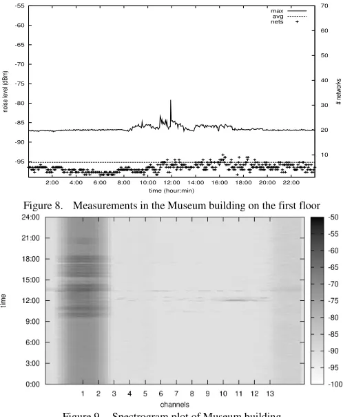
Another experiment on the first floor took place in the Museum building as figure 8 shows. The number of wireless networks found was fairly stable throughout the entire twenty-four hour measuring period. Noise levels were higher than other times at between 8am and 5pm, reaching a highest level of -79 dBm at 12pm. Average noise levels remained constant at just below -95 dBm. Most activities appeared on channel 1. The spectrogram diagram of the Museum building, as figure 9 shows, reveals wireless noise on channel 1 during the duration of the experiment.
-95 -90 -85 -80 -75 -70 -65 -60 -55
2:00 4:00 6:00 8:00 10:00 12:00 14:00 16:00 18:00 20:00 22:00 10 20 30 40 50 60 70
noise level (dBm)
# networks
time (hour:min)
[image:4.595.38.287.180.497.2]max avg nets
Figure 8. Measurements in the Museum building on the first floor
Figure 9. Spectrogram plot of Museum building
[image:4.595.308.557.342.644.2]networks were detected at one point. Noise levels also increased during this same period, reaching a maximum level of -69 dBm at around 4pm. As an exception to the findings of all other locations, the average noise levels in this location did not remain constant and showed frequent, random fluctuations, mostly on channel 10; between 8am and 6pm, the average noise levels varied among a low noise level of -95 dBm and a high level of -88 dBm. Figure 11 shows the spectrogram plot generated for the O’Reilly building, with two access points at varying distances transmitting on channels 1 and 11. The gap shown in the spectrogram is a result of slight early termination of the experiment, i.e. before the twenty-four period was completed.
-95 -90 -85 -80 -75 -70 -65 -60 -55
2:00 4:00 6:00 8:00 10:00 12:00 14:00 16:00 18:00 20:00 22:00 24:00 10 20 30 40 50 60 70
noise level (dBm)
# networks
time (hour:min)
max avg nets
Figure 10. Measurements in the O’Reilly building on the first floor
Figure 11. Spectrogram plot of the O’Reilly building
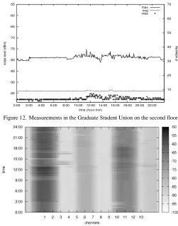
A small number of wireless networks have been found in the Graduate Student Union (GSU). This number increased after 11am, with up to nine networks found at the busiest time as figure 12 shows. Maximum noise levels in this location have varied between 10am and 8pm, ranging from 82 dBm up to -75 dBm mostly on channel 1. Average noise levels have not varied much throughout the day. The spectrogram plot gathered shows three access points transmitting on channels 1, 6 and 11, with channel 1 being most active, as figure 13 shows.
-95 -90 -85 -80 -75 -70 -65 -60 -55
0:00 2:00 4:00 6:00 8:00 10:00 12:00 14:00 16:00 18:00 20:00 22:00 10 20 30 40 50 60 70
noise level (dBm)
# networks
time (hour:min)
max avg nets
Figure 12. Measurements in the Graduate Student Union on the second floor
Figure 13. Spectrogram plot of the Graduate Student Union
On the third floor of Ussher library, between 10am and 9pm, a high number of wireless networks were found with a highest number of thirty-five as figure 14 shows. Maximum noise levels in this library only slightly increased between 10am and 7pm. Average noise levels again remained the same at -94 dBm during the duration of the experiment.
-95 -90 -85 -80 -75 -70 -65 -60 -55
0:00 2:00 4:00 6:00 8:00 10:00 12:00 14:00 16:00 18:00 20:00 22:00 10 20 30 40 50 60 70
noise level (dBm)
# networks
time (hour:min)
max avg nets
Figure 14. Measurements in Ussher Library on the third floor
B. A Summary of the Experiments
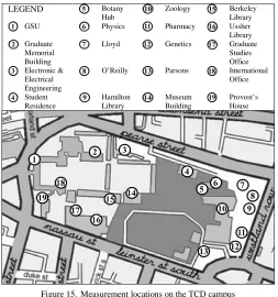
[image:5.595.305.556.53.372.2] [image:5.595.39.288.204.523.2] [image:5.595.41.286.207.361.2] [image:5.595.310.555.466.622.2]map of the TCD campus marked with the nineteen measurement locations.
[image:6.595.37.290.78.348.2]Figure 15. Measurement locations on the TCD campus
Table 1 shows a summary of all the data collected during the experiments. At a number of locations, no advertised networks were discovered, which is speculated as results of improper positioning of wireless antennas. Finding from the experiments suggest the following:
1) There is a stable average noise level on TCD campus
Evidence has shown that regardless of how high or how low the maximum noise levels were, average noise levels had a stable value at around -94 dBm all over campus with very small variations.
2) There is only one location with significant variations
in its average noise level
O’Reilly building is the only exception in the experiments where its average noise levels did not remain stable. Four obvious spikes can be seen in its average noise levels between 8am and 5pm, which might be the result of another experiment that took place in the same room, however, such conclusion requires further investigation.
3) It seems that the higher the floor, the greater the
maximum levels of noise
As data gathered from Graduate Memorial Building and Physics building (location 2 and location 6) shows, maximum noise levels at these locations had a much higher value than those of other locations. This finding suggests the idea that the higher the location, the higher the maximum noise levels. However, data gathered from Ussher Library (location 16), which is located on the third floor, suggests otherwise. Therefore, although a pattern is identified in the experiments, further studies are necessary.
4) Average noise levels have no correlation with
maximum noise levels
As one might suspect that higher noise levels could result a comparably higher value of average noise levels, the experiments have found that this was not the case. All of the graphs from the measurement locations showed that average noise levels did not vary as a consequence of the changes in maximum noise levels.
5) The number of wireless networks detected in a
location have no significant impact on the level of background noise
[image:6.595.38.289.81.344.2]One may argue that the noisier a location, the more wireless networks one should suspect. However, findings in the experiments clearly support the conclusion that there is no such correlation between the two.
TABLE I. EXPERIMENT RESULTS SUMMARY
Floor Location Max.
Noise Level (dBm)
Avg. Noise Level (dBm)
Max. No. of Wireless Networks
Avg. no. of Wireless Networks
5 -63 -93 15 4.07
7 -63 -94 66 29.36
10 -68 -93 14 2.9
11 -84 -95 29 10.71
13 -73 -94 24 11.61
15 -87 -95 29 9.24
17 -76 -94 7 2.22
Ground
19 -78 -94 4 0.87
1 -75 -94 7 2.91
4 -73 -94 17 4.68
8 -69 -93.63 33 9.54
14 -79 -95 10 4.15
First
18 -80 -94 null null
3 -63 -93 22 7.95
9 -77 -94 35 10.15
Second
12 -61 -93 null null
2 -56 -94 null null
6 -57 -94 null null
Third
16 -82 -94 35 4.25
V. CONCLUSIONS AND FUTURE WORK
Interesting patterns have been identified in the experiments, such as an almost constant average background noise throughout the day, unlike maximum noise levels. In addition, different types of noise were encountered, some of which can be traced to wireless access points, some with scattered values that must be interpreted as general background noise.
However, the data pool gathered in the experiments is not large enough for one to derive any conclusive patterns. The experiments have most importantly identified various directions for future work in the investigation of wireless background noise, which would lead to a better understanding of the effects of this phenomenon.
Although the conducted experiments have produced a good insight into the area of background noise, further research is necessary for a better capturing and understanding of the subject.
LEGEND Botany
Hub
Zoology Berkeley Library
GSU Physics Pharmacy Ussher
Library Graduate
Memorial Building
Lloyd Genetics Graduate
Studies Office Electronic &
Electrical Engineering
O’Reilly Parsons International Office
Student
Residence
Hamilton
Library
Museum
Building
[image:6.595.312.552.215.516.2]As discussed earlier, a slight pattern was discovered suggesting that more noise can be found on higher floors. However, as there are not enough measurement data to verify this indication, several test runs could be performed in the same building on different floors in order to state the validity of such speculation.
The approach taken in the experiments can be further extended to create a noise map of a whole building, rather than of sparse areas. In doing so, the measurements could be compared against a precise building structure and infrastructure, which may lead to findings with detailed explanations for noise variations. Moreover, the activities of the individuals working in a specific environment could be investigated, which again can lead to more precise comparisons, results and correlations. Further experiments can also measure wireless background noise over a longer period of time such as deploying weekly test runs which could result fruitfully in the area of searching background noise patterns in wireless networks.
A single Wi-Spy analyser that records data at every second over a twenty-hour period produces over 600 MB of data. Due to limited storage space and processing power, in the conducted experiments, data was scaled down to contain the average and the maximum of measurement values that were recorded every 180 seconds. Future studies could employ a decreased time span of every 60 seconds for example, which may produce higher resolution of the noise data and allow more precise data analysis.
Furthermore, in the deployed experiments, only the number of networks found together with the overall background noise was recorded. Future research in the area could take on the actual signal strength of different wireless networks that would vary with a changing amount of neighbouring noise. Such analysis could be produced precisely since Wi-Spy analyser measures the spectrum in a very profound way. The analysis could also study how many neighbouring channels are affected if a wireless network signal is sent over a certain channel.
What is more, actual performance measurements of a wireless network could be taken with changing levels of background noise. This can be achieved by artificially introducing wireless background noise and measuring the correlation among them, i.e., record Ethernet frame loss and the corresponding noise level during the experiment.
Finally, by undertaking these experiments, it would be possible to determine how much background noise changes valid signals’ behaviours. This would be of great use for researchers equipped with Wi-Fi devices, as they would be interested in knowing the validity of their results are in the presence of wireless background noise. As the experiment findings suggest, since a higher level of noise variations were found in buildings occupied by computer scientists, it is important that computer scientists are made aware of how
their experiments might be strongly affected by activities on neighbouring wireless networks.
REFERENCES
[1] C. Newport, “Simulating mobile ad hoc networks: a quantitative
evaluation of common MANET simulation models,” Dartmouth College, Computer Science, Hanover, NH, USA, TR2004-504, June, 2004.
[2] C. Perkins, E. Belding-Royer and S. Das, “Ad hoc on-demand distance
vector (AODV) routing,” RFC 3561, July 2003.
[3] B. Karp, H. T. Kung, “Dynamic neighbor discovery and loop-free,
multi-hop routing for wireless mobile networks,” Harvard University, May 1998.
[4] S. Lee, W. Su, and M. Gerla, “On-Demand multicast routing protocol in
multihop wireless mobile networks,” Mobile Networks and Applications Journal, Springer Netherlands, Vol. 7, No. 6, pp. 441-453, December 2002.
[5] P. Gupta and P. Kumar, “A system and traffic dependent adaptive
routing algorithm for ad hoc networks,” in Proc. IEEE 36th Conf. on Decision and Control, San Diego, CA, USA, pp. 270-283, December 1997.
[6] S. Bajaj, L. Breslau, D. Estrin, K. Fall, S. Floyd, P. Haldar, M. Handley,
A. Helmy, J. Heidemann, P. Huang, S. Kumar, S. McCanne, R. Rejaie, P. Sharma, K. Varadhan, Y. Xu, H. Yu and D. Zappala, “Improving simulation for network research,” Technical Report 99-702b, University of Southern California, March 1999.
[7] D. Ganesan, B. Krishnamachari, A. Woo, D. Culler, D. Estrin, and S.
Wicker, “Complex behavior at scale: An experimental study of low-power wireless sensor networks,” Technical Report UCLA/CSD-TR 02-0013, UCLA Computer Science, 2002.
[8] D. Cavin, Y. Sasson and A. Schiper, “On the accuracy of MANET
simulators”, in Proceedings of the 2nd ACM International Workshop on Principles of Mobile Computing (POMC'02), pp. 38-43, Toulouse, France, October 2002.
[9] S. Kurkowski, T. Camp and M. Colagrosso, “MANET simulation
studies: the incredibles”, ACM Mobile Computing and Communications Review, vol 9, no 4, pp. 50-61, October 2005.
[10] H. Lee, A. Cerpa and P. Levis, “Improving wireless simulation through
noise modeling”, in Proceedings of the 6th ACM/IEEE International Conference on Information Processing in Sensor Networks (IPSN'07), pp. 21-3, Cambridge, MA, USA, April 2007.
[11] X. Su and R. V. Boppana, “On the impact of noise on mobile ad hoc
networks”, Proceedings of the International Conference on Wireless Communications and Mobile Computing (IWCMC'07), pp. 208-213, Honolulu, HI, USA, August 2007.
[12] MeatGeek Wi-Spy 2.4 GHz spectrum analyser homepage,
http://www.metageek.net/products/wi-spy, last retrieved on 26/03/2008.
[13] Kismet Wispy-Tools homepage, http://www.kismetwireless.net/
spectools, last retrieved on 26/03/2008.
[14] Cisco Aironet 350 Wireless LAN Client Adapter homepage,
http://www.cisco.com/en/US/products/hw/wireless/ps4555/ps448, last
retrieved on 26/03/2008.
[15] Kismet 802.11 layer2 wireless network detector, http://www.
kismetwireless.net, last retrieved on 26/03/2008.
[16] Ruby programming langauge, http://www.ruby-lang.org, last retrieved
on 26/03/2008.
[17] HEAnet project homepage, http://www.hea.net, last retrieved on
26/03/2008.
[18] Live Trinity College Dublin Traffic Data Analysis project page,