On the Statistical Properties of Some Estimators of Linear System Parameters in Time Domain Analysis EUR 4480

tmkWË

EUR 4 4 8 0 e

COMMISSION OF THE EUROPEAN COMMUNITIES

ON THE STATISTICAL PROPERTIES OF

SOME ESTIMATORS OF LINEAR SYSTEM PARAMETERS

IN TIME DOMAIN ANALYSIS

by

A. C. LUCIA

• IW - f l |

1970

. \,tr tt

Joint Nuclear Research Center Ispra Establishment — Italy

LEGAL NOTICE

This document was prepared under the sponsorship of the Commission of the European Communities.

Neither the Commission of the European Communities, its contractors nor any person acting on their behalf:

make any warranty or representation, express or implied, with respect to the accuracy, completeness or usefulness of the information contained in this document, or that the use of any information, apparatus, method or process disclosed in this document may not infringe privately owned rights; or

assume any liability with respect to the use of, or for damages resulting from the use of any information, apparatus, method or process disclosed in this document.

This report is on sale at the addresses listed on cover page 4

at the price of FF 11 — FB 100.— DM 7.30 Lit. 1,250 Fl. 7.25

When ordering, please quote the E U R n u m b e r and the title which are indicated on the cover ol each report.

Printed by Van Muysewinkel, Brussels Luxembourg, July 1970.

EUR 4 4 8 0 e

COMMISSION OF THE EUROPEAN COMMUNITIES

ON THE STATISTICAL PROPERTIES OF

SOME ESTIMATORS OF LINEAR SYSTEM PARAMETERS

IN TIME DOMAIN ANALYSIS

by

A. C. LUCIA

1970

Joint Nuclear Research Center Ispra Establishment — Italy Reactor Physics Department

ABSTRACT

This report deals with the problem of determining some of the fundamental parameters of stationary ergodic random signals (mean value, auto- and cross-correlation functions, covariance functions, probability density, e t c . ) , using continuous estimators and working from time history analog records.

Within this context particular reference is made to the possibilities of the S.D.A. statistical analyzer, designed and built at the J.R.C. — Euratom, Ispra.

KEYWORDS AMPLIFIERS

LIOUVILLE THEOREM AUTO-CORRELATION FUNCTIONS

CONTENTS

Introduction pag. 5

1.) Mean value estimation

2.) Mean square value estimation

3.) Correlation function estimation

3.1.) Cross-correlation function estimation 3.2.) Auto-correlation function estimation ,

4.) Covariance function estimation

5.) Estimation of the mean value and of the mean modulus by the S.D.A. analyzer

6.) Estimation of the correlation functions and the mean square value using the S.D.A. analyzer

7.) Probability density estimation

7.1.) First-order probability density estimation 7.2.) Joint probability density estimation

8.) Estimation of the probability density by the S.D.A. analyzer

Appendix A

Appendix Β

Appendix C

C.I.) Introduction

C.2.) Programmes for D.V.M. operation

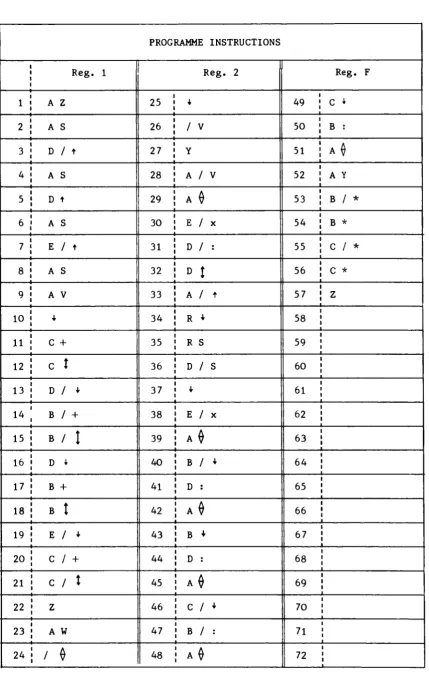
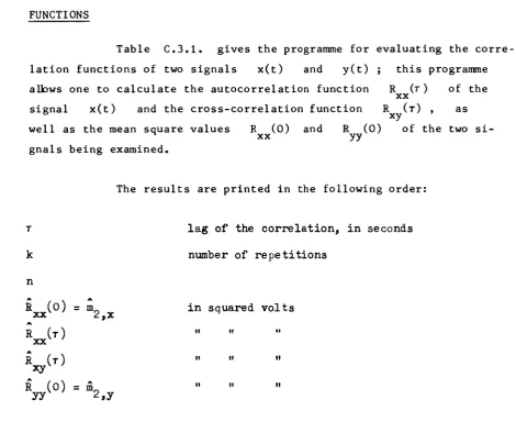
C.3.) Programmes for the calculation of the auto and cross-correlation functions

C.4.) Programmes for determining the probability densi­ ties

References

13

17 17 21

25

2Θ

4

-FIGURE CAPTIONS

Fig. 1 - Sequential operating diagram of the D.V.M. function of the S.D.A. .

Fig. 2 - Sequential diagram of the S.D.A. operation for evalua-ting the correlation functions.

Fig. 3 - Sequential diagram of the S.D.A. operation for evalua-ting the probability density functions.

LIST OF TABLES

Table C.2.1. - Programme for calculating mean values and mean absolute-values (D.V.M. function).

Table C.2.2. - Programme for evaluating the static characteristics of a system (D.V.M. function).

Table C.3.1. - Programme for evaluating auto and cross-correlation func-tions.

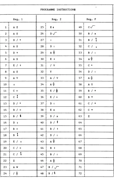
Table C.3.2. - Programme for evaluating the normalized auto and cross-correlation functions.

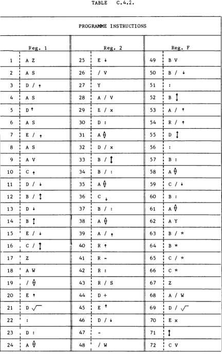
Table C.4.1. - Programme for evaluating the first order probability den-sity.

5

-ON THE STATISTICAL PROPERTIES OF SOME ESTIMATORS

OF LINEAR SYSTEM PARAMETERS IN TIME DOMAIN ANALYSIS »)

INTRODUCTION

In a previous report ) we discussed the statistical properties of continuous estimators of some functions belonging to the frequency domain (power and cross-power spectral densities and Fou-rier transforms) in the case of random, stationary ergodic signals.

In this report a similar sort of study has been extended to cover the correlation and probability density functions. A know-ledge of these functions, like that of those mentioned in the first pa-ragraph, is of great interest for the identification of systems and processes and for choosing the most appropriate and accurate

mathemati-2 3 cal models ) ).

As a particular example, the cross-correlation function has proved itself to be most helpful in studying vibration

transmis-sion pathe in installations and structures, while probability density can indicate the presence of non-linearity in the processes or systems being examined, as well as provide some informations about the nature

4 5

and the origins of the noise ) ) of system variables.

As already in the case of spectral estimators, ) the estimators analyzed here are also of a general type and constitute the algorithms upon which the operation of the S.D.A. statistical dy-namic analyzer, built at C.C.R. - Euratom, Ispra, ) ) is based.

*) Manuscript received on 21 May 1970

- δ

-1.) MEAN VALUE ESTIMATION

The mean value μ of a random variable x(t) is

8 X

defined as ) :

μχ = E(x(t)) ( 1)

but in the cases where x(t) is stationary and ergodic, one can sub­ stitute for relation (1) :

Τ

1 Γ

μχ

l.i.m. ψ

j

x(t)dt (2)

o J

T-+ °°

g in which l.i.m. means limit in mean square ) .

It must be noted that for (2) to be valid, (and together with it similar expressions ( 2 5 ) , ( 4 2 ) , ( 5 6 ) , (63) which are rela­

tive to the mean square value and to the correlation and covariance functions) it is not necessary that x(t) and y(t) are ergodic in the strict sense (strongly ergodic): it is sufficient that they are ergodic with respect to the covariance functions. Random func­ tions are said to be strongly ergodic if the equivalence of time and ensemble averages is extended to all their statistical properties. Taking into consideration expression ( 2 ) , the mean value of a statio­ nary, ergodic random signal x(t) can be estimated by using estima­ tor:

μχ

ψ f x(t)dt (3)

J _o

7­

8 Let us examine estimator (3), which is an unbiased estimator, as )

Τ

Χ>

■ Τ J * W J «

= μ

o

where we used the interchangeability property of the operation of fin­

ding the mathematical expectation and the operation of integration ),

Because the estimator we are dealing with is unbiased,

its mean­squared error is equal to its variance, which is given by:

var(/y = B(íy­ jV¿

x

) ]

2

= Ε(μ

2χ

) ­ μ

2χ

(

5

)

Substituting (3) in (5) we have:

Τ Τ

s

var(í

) = Ε Γ ­ 7

f x(t)dt

ί

χ(τ )άτ

ο ο

T T T T

= -J j j

E(x(t)x(r)) dt dr - μ

=

h i l

x x (

o o o o

Q

which gives at last ):

T

~ * V

■

?ƒ (^·ψ-)θ

β

(θ),

β

(τ)*· (7)

-Τ

-8

where C is the autovariance function of x(t) and PVV\T)

xx xx is the normalized autocovariance function, given by:

C (τ)

ρχ χ( τ ) = C (0) ( 8 )

xx

If x(t) is a real function, its covariance function is real and (7) can be reduced to the form:

Τ

varC/y = f ƒ

( ï ­^)c

(0)

(r)dr

If the autocovariance function

C ( τ )

s a t i s f i e s the condition:

xx

Τ

O

we can say that the estimator (3) is consistent, as:

lim var(£x) = 0 ( l l)

T­*oo

The condition (10) is satisfied in the case of ergodic processes ),

9­

If the integration shown in (3) is repeated k times,

and the results averaged out,the following estimator is used to deter­

mine the mean value:

k t.+T.

k¿x

T k

¿ |

>

i=1 t

where t. indicates the instant at which the i repetition be­

1

gins; this estimator, like the preceding one, is unbiased, inso far

as:

_k t.+T

E

W ■ ï ï

}_,

ƒ

X

■«*»

at

- "»

<13)

1=1 ι

as the expected value operation is a linear operator.

As far as the variance of the estimator (12) is concer­

ned, it can be obtained simply be considering the estimations û : χ,ο μ j. ; ·... μ of the mean value found in the k repetitions,

x>' Xj k

as k measured values of a random process. The sample mean is

therefore:

1 V «

lc'x ­ k

χ,ί (14)

i=1

where the subscript i indicates the result of the ±l measu­

rement.

1 0 ­

Hence we can w r i t e :

v a r

>,] ■

' Μ ­ Κ Λ ] ]

₂

■ «[(i [ «,.)']■

i=1

(Ί5)

and, by developing (15):

Κ κ

(16)

i=1

i,0=1

Ut

Remembering that for two random variables ζ and w we can write

8 ) :

E(V) =

a\

+

[

<■) j

E(z w ) =

a

rs

(17)

Ί1

a (τ)

zw

'

E(z).E(w)

P

(r)VC

(0)

(0)

E(z)-E(w) +

· ογ o

11

-be r e a r r a n g e d :

var

[ A ]

■ i [«*

['„i

] * 4 }

₊

Ψ

Λ*

? «

["„i]

I

"ij

_(T

> ­ 4

= ^ [ v ] [

1 +

*W

T )

]

i,j=1

where p..(τ) represents the degree of correlation existing between

the values assumed by the variable x(t) in the ith interval and

those assumed in the jth interval.

We can reduce (18) to a simpler, though only approximate, form:

var

[A]

­i 1+(k­l) Pk(r)

(19)

where p. .(τ) is infact assumed to be constant whatever the value: 1J

of i and j .

From (18), remembering that var(¿ .) is actually

given by the second member of (7) , we have:

lim var

T­+ °° k":

(20)

by virtue of the hypotheses already made for the case of estimator ( 3 ) , except that now the convergence is more rapid because of the divisor k ,

It can once more be seen that similarly:

12-lim var I A = O (21 )

even if Τ remains a finite value.

This is all obviously valid when p. .(Ό is less than unity. If ρ (τ) was equal to one, however, the repetitions would not have any

ij

effect, and the result would be:

var

[A]

= T a p

[V) <

22

>

as can be imagined from the fact that a p. .(τ) with identically uni-tary values would be the same thing as always making measurements over the same time interval. The most favorable situation, however, is

that of completely uncorrelated measurements, for which p. .(τ) has a value of zero, so that we have:

var

_]Λ

In order to have p. .(τ) values small enough, it is obviously neces-sary to choose the instant t. from which the measurements begin suf­ ficiently far apart.

In practice ρ, (τ ) will be greater than zero but less than one, because of which the variance of estimator (12) will be less than that of estimator (3).

In appendix A a direct procedure to evaluate the influence of the repetitions on the estimate variance is shown.

­ 13

2 . ) MEAN SQUARE VALUE ESTIMATION

The mean s q u a r e v a l u e X" of a random v a r i a b l e x ( t ) i s d e f i n e d b y :

m„ E

2,x

x

( t )

]

(24)

where the symbol m„ of the moment of the second order is introduced.

¿ ,x

If x(t) is stationary and ergodic, we can write:

"2.x

l.i.m. Τ ­* °°

l(t) dt

(25)

Let x(t) therefore be a stationary ergodic random signal; its mean

square value can be evaluated by the estimator:

m, _{2,x Τ} 1

\t)

dt

₍₂₆₎

which i s unbiased, since i t s expected value i s given by:

m,

!,xj

_TJ

E

' ( t )

dt

=

m

₍₂₇₎

Let us now look at its variance (equal to its mean­squared error, owing

to unbiasedness of the estimate) :

var

J

5,x]-[

E

p2,xJ]

2

=

Β

[

Α

!,χ]-«ί,χ (28)

1 4

-from which, introducing (26) and carrying the mathematical expectation operation inside the integration operation, we obtain:

var m _{2, χ}

.Τ .Τ

1

[

Γ

=

7· Ι

ο ο

Xa (t) χ2(θ) dt do -

]

Remembering now the expression relating the mathematical expectation of the product of four normal random variables to their correlation functions and mean values ):

E χι X2X3X4

] =

1 2

34

13

24

14

23 -

*ί *e *a *4

we can rearrange equation (29) , so t h a t i t becomes:

var

_{2,χ J}

Τ Τ

L. f f

m2

R2 ( o - t ) dt d0 - 2 μ4

χ χν χ

(3θ

o o

If we wish to express (31) in terms of the autocovariance function C (τ) and to resolve p a r t i a l l y the double i n t e g r a t i o n , we have f i n a l l y :

var

_{!_}

_{2,xJ = T}

-T

1 -

¡■^ΛΓ C

(τ) +2 μ» C (τ)

dT (32)

If

x(t)

i s real:

15-In both cases the variance tends to zero if Τ tends towards the in­ finite, always presuming that the autocovariance function and its squa­ re are absolutely integrable; if this is so, then:

lim var

Τ*»00

M

(34)

namely, the estimator is consistent.

Where the measurement is repeated k times and the k results are averaged out, the estimator takes the form:

ι ran

k 2,x

k t.+T

τ i £ ƒ

x3

<

t} dt

i=1 *i

(35)

where t. is the instant at which the i repetition commences, _ι This estimator is also unbiased:

E

[A,] - Hyf'-h»

(36)

while as far as its variance (equal to its mean-squared error) is con­ cerned, what we have already said about the mean value estimator is va­ lid. One has, in fact:

κ

var

[k

Ä

2,x] =

ÏÏ[

+

kT

Ì J

] ·

(37)

i,j=1

where var m_ . represents the variance of an estimate carried out by a single measurement, and is given by expression (32).

16­

By assuming ρ. .(τ) to be constant whatever the values

of i and j , we can write the approximate, simplified expression:

var

[A.,]

1+(k­1 )pk(r)

(38)

The less the different measurements are correlated, the greater is the

efficiency of the repetitions in reducing the estimate variance.

Where x(t) has a mean value of zero, (38) becomes

(if x(t) is real) :

var _km2,x

1+(k­1 )pk(r);

it­ σ<

τ

!

(T­r)

dr

(39)

where the autocorrelation function R (τ) has been expressed as:

R

xx^

^

χ '

^

^

W ' P(

)

It will be observed that, if x(t) has a mean value of zero, the moment

of the second order, or mean square value m , coincides with the

¿ ,x variance σ 2 ,

χ

In the S.D.A. statistical dynamic analyzer the estimation

of the mean square value is done on the basis of estimator (35); more

17

3.) CORRELATION FUNCTION ESTIMATION

3.1.) Cross­correlation function estimation

Let us consider two random variables x(t) and y(t) ; 11 12

their cross­correlation function is defined as ) ) :

R (τ) = E x(t) y(t+r)

xy j_

(41)

If the variables are stationary and ergodic, the cross­correlation func­ 13

tion may be computed by a time average, that is ):

a (τ)

xyv

'

x

l.i.m. ^ / x(t) y(t+T) dt Τ ­» oo l J

(42)

Therefore, as in the case of mean square value, the estimator of the cor­

relation function of two real ergodic stationary random functions can

be provided by:

a (τ)

xy

*

=

i

x(t) y(t-n-) dt

(43)

where Τ is a sufficiently long period.

Let us look at the properties of this estimator. We find:

E

â (τ)

1

ƒ EJ~x(t) y(t

+

r)"j

a (τ)

(44)

that is, it is not biased.

18

-Its variance (equal to its mean-squared error), defined as:

var

£ (τ)Ί

xy

"ι

i s given by:

var

Τ Τ

EV>]

■

?l

ƒ

o o

x(t) y(t-n-) χ(θ) y(e+r) dt

dø - R

(r)

(46)

Expression (46) shows that, in order to evaluate the variance of the estimator of the cross-correlation functions, knowledge of the correla-tion funccorrela-tions is not sufficient; it is also necessary to know moments of higher order.

Nevertheless, when the random processes under examination are normal processes, the moments can be expressed in terms of mathema-tical expectations and correlation functions. In general, for four normal variables x1(t) , x_(t) , x (t) and x,(t) ,

expres-sion (30) has been proved. In the present case we can write:

xx(t) = x(t) ; ,

Xa(t) = x(0) ;

*a(t) = y(t+r)

Xi(t) = y(0+r) (47)

- re

τ τ

var

[ V

_{T )}

] ■

JS

Jl4y<*> ♦*«<»­*> V'­*» *

+ R (ø+T­t) R ( ø ­ t ­ r )

xy

yx

2 μ

μ

1 dt dØ ­ Η

(τ )

(48)

which, when developed, gives us the expression we are seeking:

varper)

Τ

=

* /

T

(

1

"

i

î

L

)[

R

­

(

"

)

v » >

+

V "

+ T )

V

C

"­

T )

"

- 2 μ2 μ2

Mx My

₍₄₉₎

or, in terms of covariance functions:

var

χ

[>

t T )

]

=

* /

T

(

1

" * )

l°**

M

"¿

η)

* V"

+T)

V

(

"-

T)

]

χ

*

ƒ (

1

" ^ ) fa

0

»

+

Φ**

*

v / > ) ♦

+

ν

°νχ

"

^

Therefore» where C ^ , C , C^'Cyy

·

yx

absolutely

integrable, (5θ) allows us to w r i t e :

lim var

T-*°°

LV>]

20

which means that estimator (43) is consistent.

Formula (50) is quite complicated and it is often rather difficult to prove that relation (51) is satisfied. For practi­ cal purposes it is therefore more convenient to observe that (51) is proved if the covariance functions C > C , C , decrease

in-v xx yy xy

definitely in absolute value as \τ\ tepds to infinity.

We repeat that stationary random variables x(t) and y(t) which satisfies relations (10) and (51) are said to be ergodic with respect to the covariance functions.

If we consider the estimator relative to the case of k repetitions for the cross-correlation function too, it can be expressed as:

vR (r)

k xyv

1 1

k Τ

k t.+T

ι x(t) y(t+T) d

(52)

i=1

which is unbiased, as:

k t.+T

E

kV')

ι

ι

k Τ

i=1 *i

x(t) y(t+T)| dt

_{R^ir) (53)}

while its variance can be expressed as a function of the variance of esti­ mator (43), of the number of k repetitions, and of the degree of correlation Pir(T) existing between the k measurements; the for­ mula is the same one already seen in the case of the mean value and mean square value:

var

J

(τ)

1+(k-1 )pk(r)

21

-the considerations already made for relations (19) and (38) beeing also valid for expression (54).

3.2.) Auto-correlation function estimation

What we have said about the cross-correlation is substan­ tially valid also for the autocorrelation function.

The autocorrelation, defined for a random variable x(t) by :

R (τ) = E

XXs

x(t) χ(ΐ+τ)

(55)

can, if x(t) is stationary and ergodic, be expressed as

R (τ)

XX

l.i.m. - /

Τ -+ » J x(t) x(t+T) dt

(56)

for which one can in practice use the estimator:

R (τ) =

XX

X

1 Í x(t) x(t+r) dt (57)

to estimate the autocorrelation function of an ergodic random variable,

This estimator, like that of the cross­correlation function, is unbia­

sed:

E

J

] ■

*ƒ

E

while its variance is given by the expression:

­ 22

Í>

( T )

J

= ?

ij

1

--)

*

(»?) a j v T i g . K )

(59)

which can be obtained rapidly from (49) by substituting the variable χ for the variable y .

In terms of covariance functions, the expression of the variance of the estimate of the autocorrelation function is obviously similar to expression (50), from which it is obtainable by substitu­ ting μχ for μ . and C for C and C .

y xx xy yy

As far as the consistency of the estimate is concerned, what we have said for the cross­correlation function is also valid; the relation which expresses this consistency:

lim var T­*°°

[

R (τ)

xx^ (60)

i s p r o v e d i n t h e c a s e where C and C2 a r e a b s o l u t e l y i n t e g r i l e ,

r x x XX J O

An e s t i m a t o r which t a k e s i n t o a c c o u n t k r e p e t i t i o n s of t h e m e a s u r e m e n t s c a n a l s o b e c o n s i d e r e d f o r t h e a u t o c o r r e l a t i o n :

J

(τ)

k xxx

k t.+T

■ k τ

ν ι

*(*)*(*■"■>

dt

1=1 1

(61)

For the properties of this last estimator we can refer back to what was said about the cross­correlation functions.

23

4.) COVARIANCE FUNCTION ESTIMATION

Let us consider the usual two random variables x(t) and y(t) ; the cross-covariance function is defined as:

C ( τ )

xy ' E x ( t ) - μ. y(t+T)

[[»

-ν]]

o r , i f the v a r i a b l e s x ( t ) and y ( t ) a r e ergodic with r e s p e c t to the covariance f u n c t i o n s (weakly e r g o d i c ) :

G ( τ ) xy

τ

l . i . m . ψ / x ( t ) - μχ

τ -» °° J L _

Λ dt

₍₆₃₎

The c r o s s - c o v a r i a n c e e s t i m a t e C ( τ ) can consequently be defined b y :

xy

C (τ) _xy

1

_τ

_-4)

(64)

In practice the effective mean values μ and μ of the variables x(t) and y(t) are replaced by the estimated mean values μ and μ ; because of this the following estimator is the one actually

J"

used:

C (τ) _xy ψ / x(t) y(t+T) dt - μ ·μ

x y

(65)

which means that the cross-correlation function R and the mean * y

v a l u e s μ and μ are measured s e p a r a t e l y , and from t h e s e

•J

measurements the c r o s s - c o v a r i a n c e i s then deduced:

CW( T ) = R ( τ ) - μ * μ

xy xyv *x y

(66)

2 4

-Let us now look at the properties of this estimator. As far as the bias is concerned, we have that the expected value for the estimate C (Τ) is given by:

xy ° J

E

"c (τ)Ί

xy J

E

χ y

(67)

which, rearranged on the basis of what we said about the estimates of the correlation function and of the mean values, becomes:

T T C (τ)

xy

V

r )

-?/ ƒ

E

x(t) y(0) dt d0 o o

(68)

and finally gives:

E

"c (τ)Ί

_V

_{T )}

_{- Ï}

1

ƒ e -

\n\

\

T

)

°xy

-Τ

(69)

Hence C (τ) _xy is a biased estimate of the cross­covariance function

C (τ)', its bias is given by:

xy ' ° J

ï

bias C (τ) xyv

-τ

0

lì

τ

If however the cross­covariance function is absolutely integrable, the

right hand member of equation (70) tends to zero when integration

time Τ tends to infinity, so that we haye:

lim bias C (τ)

25

which means t h a t :

lim E

Τ·+°°

0W

(T)

]

C (τ)

xy

(72)

so that we can say of the estimator under examination that it is unbia­ sed in the limit.

It is clear from (72) that the estimated value C ( τ ) xy can assume the true value C (Τ) only by taking the measurement

xy

time to infinity. But it is also obvious that if one could replace the estimated mean values μ and μ by the true mean values μ

Λ jr Λ

and μ in (65) , then the estimator would be unbiased.

In order to see now whether or not this is consistent, it is necessary, on account of the bias, to evaluate the mean square error and not the variance. The mean square error (m.s.e.) is defined by:

m.s.e.

[y*>]

E

"c (τ) - C (τ)Τ ]

_xy

_{xy J j}

(73)

or, in terms of the variance and the square of the bias:

m

re (

|_ xy

. s . e . C_ ( τ ) _{v a r}

[V>]

"c

(τ)Ί

xy J

(74)

where the bias of the estimator has the expression we gave in equation (70), while the variance of the estimate can be evaluated on the ba­ sis of the definition;

var

_{. ** J}

β (r)l

E

e

(τ)

xy

']'H»[V>]Ï

(75)

26­

The strict development of expression (74) is given in appendix B,

for the sake of accuracy, but it has no effective or practical interest

because the final expression is too complex. For this reason it

is convenient in practice to construct a simplified form of this expres­

sion, even if it is only approximate, by replacing the mean estimated

values μ and μ by the mean values \i and μ *

x y χ y

This does not lead to a significant error, since the variance of the

estimator of the mean value is rather small.

Ignoring thus the difference between the estimated mean

values and the effective mean values, estimator (65) can be written

as:

Τ

Ô

xy

( T )

= Τ

ƒ [

X(t)

-

μ

χ] [

y(t+T)

*

M

y]

dt

<

76

)

o

which gives an unbiased estimate of the cross-covariance function, so that the mean squared error of the estimate becomes:

m.s.e.

[V

_T)

]

_{■ ™ [V}

_T)

_{] ■}

_E

_{[ [ V}

_{T )}

_{] '] ­ °^}

_(τ)

_<??>

On the other hand we know that:

Τ Τ

f pxyÍT jT j = ^T

ƒ ƒ Ε Γ ΓΧ( t )-μΊ (~y(t+T )-μΊ Γχ(0 )-μΊ Γν(0+τ )-μ J d t

dØ =

Τ

%^

?ƒ

τ

(

1

-

ψ)

[C>)C>)

♦ C

xy

(n+r)

Cyx

(^)] dn

27-for which the approximate expression of the mean square error of the cross-covariance estimator becomes:

m.s.e.

[V>]*

*ƒ

0-Ψ)

r

_xx^

_yy

_V^V^

(79)

dn

which, if x(t) and y(t) are ergodic, tends to zero if Τ tends to the infinite.

As far as the autocovariance function is concerned, every­ thing that has been said for the cross-covariance is valid.

The relative formulae can be obtained immediately from the analogs given for the cross-covariance by substituting x(t) for the variable

y(t).

28

5.) ESTIMATION OF THE MEAN VALUE AND OF THE MEAN MODULUS BY THE S.D.A. ANALYZER

The S.D.A. statistical dynamics analyzer evaluates the

mean value and the mean modulus of the x(t) and y(t) signals

being examined,on the basis of estimators:

k ti+T

μχ

=

¿ Y

V

ƒ x(t) dt (80)

t.

i=1 ι

k

t

T

dt (81 )

i=1 "i

and on the basis of the similar estimators relative to variable y(t), The quantities ο, , β. » *^ and &"£ supplied by the analyzer to the computer which carries out the averaging and the normalizations on them, are given by:

t.+T t +T

ι Λ Γ i

α.

Ι

f

(t) dt =

¿ i x(t) dt (82)

*i *i

t,+T t,+T

/51 = / |fx(t)| dt = ¿ / |x(t)| dt (83)

t.+T t±+T

29

t.+T t.+T

δ- = ƒ

|f

(t)|dt = ! ƒ

|y(t)| dt (85)

t. t

where f (t) and f (t) are the output frequencies of the voltage _{x y}

to frequency convertors of the χ and y channels respectively, and | f (t)| and |f (t)| are the same frequencies taken always with a positive sign; the proportionality coefficient of the voltage to frequency conversion is indicated by h .

Finally the analysis time Τ is equal to η times the unity Τ of machine time, equal to 10 milliseconds:

Τ = η Τ _m

while the instant at which the ith repetition starts is indicated by t. . From the abo>

(82) .... (85) , we have:

by t. . From the above, and on the basis of (80) , (81) and

μχ

k . k

k

n V

)

i

Å/

"i

m L— i—

i = 1 i = 1

(86)

μ

χ k η T

m

*>Ί - ΐτ7"ι <

87

>

i=1 i=1

k , k h

1 1 v \ y _y.

μγ = k n T h / y i = η k / * i

J m Í—J '—i

V

r

(88)

' I

i=i i=1

h k

"β,

=

T ^ Y V

(89)

M

|y|

/ .

i

m

i=1 i=1

30

The h factor which appears in expressions (86) to (89) is the normalization coefficient of the S.D.A. when operating as a di­ gital voltmeter (D.V.M.) ) and is equal to:

hv = — (90)

m

In the D.V.M. operation, the S.D.A. apparatus can be employed to obtain the static characteristics of a system.

In fact, if x(t) is the perturbation signal sent to the system or process being examined, and y(t) is the reply of the system itself, one can obtain, point by point, the static characteristics A of the system by giving to x(t) a step by step behaviour:

I

( 9 1

>

The averagings performed on χ and y serve in this case to reduce the influence of spurious noise which is superimposed upon the useful signals. We can write:

7'i

A = -r = -Z = (92)

Χ μ k

Mx _{α .}

ι i=1

31

-ANALYZER

— »

COMPUTER

Read and store

V

*i'

i'

*i

i

Calculate Σ α.

1

Calculate Σ

β.

i

Calculate Σ

Χ

i

i

i

Calculate Σ δ.

i

Γ

1

Read and store

h , n, k

ν '

'

Ι

Calculate Τ

Ι

Calculate

x ( t )

J.

Calculate

| x ( t ) |

Fig.1

Calculate

y ( t )

I

Calculate

| y ( t ) |

­ 32

6.) ESTIMATION OF THE CORRELATION FUNCTIONS AND THE MEAN SQUARE VALUE

USING THE S.D.A. ANALYZER

The mean square value, and the auto and cross correlation

functions are evaluated by the S.D.A. on the basis of estimators of

the type (35), (52) and (61); in particular»

Vf

m2,x

H£/

x9(t)dt

(93)

i=1 *i

4. n

k

V ?

*χχ

(τ)

- ï » E

/

X(t)x(t+T)

dt

(94)

i=1 *i

V?

ν

( τ )

- k ïï^

ƒ *<*>*<*«*)« (95)

i=1 *i

where as usual k indicates the number of repetitions, while the ana­ lysis time Τ is expressed as the number of cycles of the reference generator frequency ):

* - ?

The lag τ of the correlation functions is given by ):

τ = 2f

­ 33

Let us take the case of the mean square value m , ¿ ,χ

i.e. the autocorrelation of x(t) for a lag of zero.

The input signal x(t) , after having been led to dynamic 2A by

amplification, is sent to two level—comparators and compared with two

mutually independent reference voltages (one with a saw­tooth form,

and the other one randomly variable and equiprobable on 2A ) , such

that the probabilities P1(t) and P~(t) that x(t) will be

greater than the first and second comparison voltages respectively are 14

equal ) . These probabilities are proportional to the amplitude

ft 19

of the signal x(t) under examination ) ):

Pl

(x) = P

(X) =

-^

T

—

(96)

where 2A is the dynamic, in amplitude, of x(t) after having

been amplified.

The probability that a logical exclusive­or operation applied to the

logical output voltages of the two comparators will give a positive

result, is equal to:

Pp = Pi(x) 'Paix) +|l ­ Ρ Ι ( Χ ) Ί Γ Ι - Pa(x)| (97)

while the probability ρ that the result of the exclusive or opera­ tion will be negative is equal to:

P

= Pi (x) M - Pa (x) + Pa (x) 1~Pi(x)

(98)

Introducing the expression given in (96) for p..(x) and p9(x) we find:

Ρ

x

(t) + A

p

2A

(99)

A

- x

(t)

2A

P n OA» (100)

34

A bidirectional counter placed after the exclusive or circuit gives

us a measurement of the difference between the time during which the

output of the exclusive or is positive (positive count) and the ti­

me during which it is negative (negative count) .

This time is given by the difference between the two probabilities

ρ and η :

x2( t )

Pp ­ P

¡ 2 ~

(101)

where the time is given in relative units, as a fraction of the total

analysis time.

It is measured by the bidirectional counter, by means of pulse counts;

if f is the timing frequency, we have:

If we consider all the bidirectional counters, their contents α. ,

β. , ï. and δ. are given bys

t.+ n/f

«i

=

[

J È Í Í L f

dt

« J­ .9 t

t.

1

t.+ n/f

/?. = ! x(t)x(t4T) f d t

Jt . A2 t

ι

(103)

(104)

t. + n/f

r f x(t) y(t+r) a t ( 1 0 5 )

- 35

δ.

1

ti + n/f

ƒ

- ^ -

t

(106)

X ·

because of which, considering the case of k repetitions, and taking (93), (94) and (95) into account, we can write the following rela­ tions which evaluate auto and cross-correlation functions and mean square values by means of α. , β. , X. and δ. S

m _{2 , x f. k n} A

,L.

1 L \

Y't -

ι_ ι r \

ζ Η I>i

i=1 i=1

k k

*»<*>-

A3

f; H y^i = r H ^ i

i=1 i=1

R

(τ)

= A

1-

¿ £

V r .

*y

t

Z-.

*\

(109)

h k n / i c

i=1 i=1

m2

K. Λ

„ 1 i f Γ,

l ì

f Γ.

,y

f

k n / _

i

h

k n ¿^

i

(110)

i=1 i*1

The normalization coefficient h introduced in the right hand mem­ c

bers of (107) ....(110) is given by:

where f. varies from decade to decade, and A is equal to 10 volts.

X

36

If we wish to obtain the normalized correlation functions,

in such a way that they vary between a maximum of one and a minimum of

zero, the formulae become:

m _{2,x h} 1_

1 1

i=1

(m)

R ( τ )

χ χχ

R ( o )

χ χ ^

R ( τ )

X X

m _{2 , χ}

»

i=1

i=1

(112)

R ( r ) xy

R ( 0 ) . R ( 0 )

xxx yy

R ( τ ) xy

2 , x 2 , y

m _{2 , y}

- i n

fv

h k n / i

C _i=1 L—

¿Λ

i=1

^i-E

s

i

i=1 i=1

(113)

(114)

In fig.2 a sequential diagram of the S.D.A. analyzer opera­

tion for calculating the correlation functions is shown. The operations

performed by the computer, which constitutes the final element of the SDA,

are listed separately from those performed in the upper section, called the

analyzer, and which carries out all the elaborations on the signals to be

examined.

3 7

-ANALYZER

COMPUTER

i = k

Fig. 2

Read and store a

i ' V

i ' *i

I

Calculate Σ o . Calculate Σ β.

i *■

I

Calculate Σ ϊ:

I

Calculate Σ δ.

i i

J

1

Read and store hQ, f, n, k

i

Calculate τ

ι

Calculate R (0) _xxN

i

Calculate R (τ)

XX

i

Calculate R (τ) xy

1

Calculate R (0) yy

i

­ 38

7.) PROBABILITY DENSITY ESTIMATION

7.1.) First­order probability density estimation

Given a random variable x(t) , the first order probability

density ρ (£) is defined as:

χ

Τ

p

x

(

^ =

l™ h l ì

dT

' = i

iffl

k

f

(113)

Δχ­»ο Δχ­»ο

where Τ indicates the measurement time, T' the total time during

which, in the course of the measurement, the variable x(t) has as­

sumed values between ξ- αχ/2 and ξ + Δχ/2 , and finally Δχ

is the amplitude of the window centered on the value ξ under exami­

nation.

The estimator of the first order probability density can

thus be the following:

P.(i) -

h;

Ï

ƒ «'

.T

1 T'

xs Δχ Τ J Δχ Τ (116)

o

The expected value for the estimate ρ (ξ) is given by:

E

>«>] -

h

_E

[ f ]

■

h**(t*-f)

where ρχ(<? + Δχ/2) i n d i c a t e s the pr b a b i l i t y t h a t the value of x ( t )

w i l l be w i t h i n the amplitude window Δχ c e n t e r e d , as already s a i d , on

- 39

ί+Δχ/2

P x ( ^ f ) = ƒ Ρχ<*>*> (118)

ξ-άχ/2

Expression (117) tells us, therefore, that generally estimator (116) is biased; the value it gives is not in fact precisely ρ (ξ) , but the mean of the values it assumes for values of x(t) included bet­ ween ξ - Δχ/2 and ξ + Δχ/2 .

This bias can obviously be reduced by reducing the window amplitude ^x On the other hand, estimator:

»x(«**)

■

*ƒ

dT

'

■

Τ

is unbiased, as its expected value is:

■[«.(<*¥)] ■

E

[fj ■ *(<* τ

(119)

(120)

i.e., it gives us precisely the integral of the probability density inside

the amplitude window.

The mean square error of the determinations carried out by

means of estimator (116) is not easy to evaluate, but can be expressed

fairly approximately by the following relation ):

Aa pfte) / ΔΧ a3 P _ t è ) \ 2

r ­ , A* p­tfj / ΔΧ 9' VXKÇ}\

Γρ

(^)Ί = * — —

♦(

T a — )

L

J

Β Τ Δχ

ν (ξ

)

\ 24

Η

/

(121)

where the two terms of the right hand member represent the variance of the

estimate and the error contribution due to the bias respectively.

In expression (121) , Β indicates the bandwidth of signal x(t) in

40­

examination, and Τ indicates the total analysis time; A repre­

sents a constant whose value is linked to the nature of signal x(t)

and for which the value of 1/v~2~ can be assumed where x(t) has

a uniform spectrum within the frequency range Β ) .

The above mentioned expression shows that the mean square

error does not cancel out when Τ tends to the infinite, inasmuch

as the error due to the bias remains; the estimator is consequently not

consistent.

The mean square error cancels out only when Τ tends to

the infinite and Λ.Χ to zero, as long as the product Τ.Δχ also

tends to the infinite. In practice, however, the second derivative

of the probability density of the signals most often encountered is

small, so that when Δχ has been fixed at a sufficiently small value,

the contribution due to the estimator bias can be ignored.

When the determination of the probability density is per

formed on the basis of k measurements, the estimator becomes:

Λ<«>

^­ T'

­ \ i (122)

k ) Δχ T. K¿¿>

i=1

Also in this case the estimator is biased :

i=1 i=1

while the effect of the k repetitions on the variance of the estimate

is similar to that already seen in the case of the mean value determina­

tions or of the correlation functions.

41

-var

íJ* )

A3 p3^ )

Β Τ Δχ ρχ(ί)

^ _ ιΓ

1 +

ι Γ .

( τ

) Ί

6

Cê)

kL

¿

J

i,J=1

Vi

or, if for purposes of simplicity we suppose p. .(τ)

in spite of variations of i and j :

(124.)

t o be c o n s t a n t

v a r

[A«>]

A3 P3^ )

Β Τ Δχ px( e )

( k ­ 1 ) p. ( τ ) + 1

( 1 2 5 )

where for p. .(τ) and Ρν(τ) the comments already made in previous

chaptea are valid.

7.2.) Joint probability density estimation

Given two random variables x(t) and y(t) , we define

the function:

p

x , y

^ '

τ 1 1

τ-*» Δ χ Ay

Δχ­>ο ày*o

'1

1 1 dT" = l i m TT TZ

m tl

Τ-+°° Δχ-*ο A y * o

Δχ Ay Τ (126 )

as joint probability density.

In relation (126) Τ is the total analysis time, while T" re­

presents the overall time during which, in the course of the measurement,

the value of the variable x(t) happened to fall within the voltage

window Δχ, centered on the value £, and the variable y(t+τ)

fell in the window Ay centered on the value η .

As joint probability density estimator the following can thus

be adopted:

- 4 2

τ

1

1

1

Γ

1 1

Τ"

P

y t e , " , T )

= Αχ" Ay" Τ J

"

Αχ" Ã7 "Τ

(127)

which i s a biased e s t i m a t o r , inasmuch as the operation of mathematical

expection g i v e s :

E

[V*.-.*)]· fe fc«[¥]-

k

fe»,„(<**.'*

_A

í.*)

(128)

where the n o t a t i o n

ρ

( ί ± ~ , η + - ^ , τ ) represents the

p r o b a b i l i t y t h a t the x ( t ) variable i s included between the value

ξ

-

ψ

and the value

ξ + ψ ,

and the y(t+r) variable b e t ­

ween the values η -

-τ~

and η +

-g- '

ξ+άχ/2

n+Ay/2

Χ 7

ξ-àx/2

n­Ay/2

(129)

The mathematical expectation of estimator (127) does not therefore

give us the exact value of the joint probability density, but the mean

of the values assumed by it for values of χ included between

ξ ­ Δχ/2 and ξ + Δχ/2 , and of y included between η ­ Ay/2

and η + Ay/2 . The bias of the estimate can therefore be reduced

by adopting narrow windows Ax and Ay .

The estimator of the integral value of the joint probability density

inside the above mentioned amplitude windows given by the expression:

43 ­

is, on the other hand, unbiased, as is evident from

(129).

It is exceedingly difficult at this point to obtain the mean squared

error of an estimate performed by estimator

(127), or its variance,

by strict methods.

If we suppose windows

Ax

d

Ay

to be

sufficiently small, the error due to the bias can be ignored, and the

mean squared error and the variance can be considered to be equal; then,

where

x(t)

and

y(t)

are both signals with limited frequency

bands

Β

and with uniform spectral behaviour within this band, we

can adopt for the variance of estimator

(127)

the expression

) :

var Ô

(¿,η,τ)

=

&*

(131 )

LX , y J Β Τ Ax Ay P _ _ ( £ , T 7 , T )

where

C

is a constant.

In the case of measurements repeated

k

times and averaged out, the

estimator of the joint probability density becomes:

,—^ Φ«

(*

\

1 V 1- i_ i

i=1

while its variance can be expressed as:

C

p£

(ξ,η,τ)

(k­1) p

(r·) +1

var

[

k

P

x>y

(e,",T)j =

B Τ Ax Ay

ρ

(ί,η,τ)

(133)

where for the ρ, (τ') function, the considerations made in the

case of the first order probability density are valid .

4 4 ­

8.) ESTIMATION OF THE PROBABILITY DENSITY BY THE S.D.A. ANALYZER

1 I ι 1 1

The first order probability density ρ (ξ) and the joint

probability density ρ (£,η,τ) are evaluated, in the S.D.A. analy­ x»y

zer, on the basis of estimators of types (122) and (132) , which

are used in the form:

.+f/n

5

ej)

. ι y

1 .

1

¡

χ

dT!

*x * k / Δχ η ƒ ι

(134)

1.1 ri

k T±+f/n

Ρ (ξ,η,τ) = τ y ΊΓ ΊΓ - ! <*TV (135)

^x,y^ ' " k / Δχ Ay η / i

i l l

i

where the analysis time T. of each of the k measurements is expres­ sed as:

η

Ti = f

f being the frequency of the reference generator ) and η the number of integration cycles which assumes here the significance of time extension factor ) .

The lag Τ of the joint probability is given by ):

1 T = 2f

Let us look now at the significance of the quantities α. , β. , ί'. 7

and δ. supplied by the analyzer ):

*i =

1

°"

3

ƒ

X

τ.

1

T.+n/f

­ 4 5 ­

1^+n/f

ß± = 10"3 f ft xc(t) dt (137)

Ti

T.+n/f

'i

° "

i

t

o(

^

c ( ^

i

/ '

T.+n/f

*i =

"

ƒ

n '

Ti

where by £ and η are indicated the voltage levels (relative to the variables x(t) and y(t) respectively) at which we per­ form the measurement, while f¿ and f are the frequencies cor­ responding to these levels after the voltage to frequency conversion:

f

= £

ξ h

η h

h being the proportionality factor for the said conversion.

Then the output of the window comparator to which the si­

gnal x(t) is sent (together with the reference voltage ξ ) is

indicated by χ (t). Function χ (t) is defined by:

c c

Ax /^\ ,. Δχ

Χ (t) = 1 if ξ - ψ < x(t) < ξ + ψ

c

χ (t) = 0 elsewhere

C

because of which:

46-i+n/f

x j t ) dt = T!

i c" ' i (140)

T,

Function χ (t) , delayed of a time quantity Τ , is indicated by χ (t-τ) , while y (t) represents the output logical voltage of the window comparator to which signal y(t) is sent together with the reference voltage η .

Function y (t) is defined as: c

yc

(t) = 1 if

η

- 4ft < y(t) < 1, + 4jE

y (t) = 0 elsewhere

C

so that we have:

T.+n/f

/

τ.

1

xo(t-r) yc(t) dt = T- ( 1 V I )

Finally, f is the timing frequency according to which the times (measured by pulse counting) are measured. From everything that has been said, we obtain:

n/f Ti+

-«. = IO"

ƒ

¿ d t = £ f IO"

(

2)

τ.

1

T

n / f

/3

=

10""

f

f

x

( t ) d t

= 10"

f

T'

= 10~

f

~ ρ

( ^ ) Δχ

τ .

4 7

-T . + n / f

=

10"

f. /

χ ( t - r ) y ( t ) d t

=

10~

f. T

1 VI c c t

T .

1

10"

f^ f P

y(e,Tj,T) Δχ Ay

(144)

T j+ n / f

> 4 = 1 U If a t = Γ 7 Ί υ ^ . c \

i

/

h h f (145)

10"

f'

? dt =

?■ S 10

τ.

1

From these expressions we can then obtain the following r e l a t i o n s which

give the f i r s t order and j o i n t p r o b a b i l i t y d e n s i t i e s , as well as the v o l ­

tage levels at which we are performing the measurements, in terms of the

well known q u a n t i t i e s

α. ,

β.

,

ï.

and

δ. :

h

i=1

1=1

Ρχ

f

k°n Δχ

)_fi

7" Δχ"

Ä )_ƒ 1

(146)

(147)

i=1 * i=1

k k

\·3

/ . s 10^ V^ j _ J__ __f_ ^7 y

P

x,y^

f

k n Ax Ay

/_ /i

*

ixiy kn

¿_ 'i

(148)

i=1 v 1=1

3

h 1 0 f Ν δ

Λ.

1-

-£-

V e

i h k η / i

k η

[_

i

h

k η

/

i

(149)

1=1

1=1

In expressions

(146) to (149)

two different normalisation coeffi­

­48

That of the probability densities is indicated by 7

and depends upon the timing frequency f ) : cients appear.

, *

10

while the normalisation coefficient relative to the reference voltages

ê and η depends upon the value of the proportionality factor h

of the voltage to frequency conversion ) , and is indicated by h

10

For purposes of accuracy the values of the two coefficients in the six

frequency decades ) are here listed:

Decade h Ρ h* Ρ I 0,01 0,39262 II 0,1 3,9262 III 1 39,262 IV 10 392,62 V 100 392,62 VI 100 392,62

From the above table of values it can be seen that:

h* = h . 39,262

Ρ Ρ

h* = 10 . 39,262

if h S 10 Ρ

if h > 10 Ρ

Therefore, having stored the values of h in the normalisation coef­

7 17 P

ficient diode matrix ) ) , it is possible to obtain the values of

h from those of h by means of an appropriate calculation program­

me (see Appendix C4).

A sequential diagram of the S.D.A. operation for calculating the proba­

4 9

-ANALYZER

COMPUTER

Read and s t o r e α . ,

ßiJ**

$t

Calculate

Σ ο .

i

i

I

Calculate Σ

β.

I

Calculate Σ

ï>

I

Calculate Σ δ .

i

i

Read and store

h , f, n, k

Ρ

I

Calculate

τ

I

Calculate Τ

I

Calculate

ξ

Calculate η

h >10

Ρ

I

h «10

Ρ

1

lv* « 10.39,262

C a j _{Lcuiate ρ}

h* =

Ρ

, t e )

h

Ρ

•39,262

I

Calculate

P­^Cí »Π,

)

I

Fig. 3

Print Results

50­

APPENDIX A

Given a stationary ergodic random signal x(t) , let

us consider the estimator μ of its mean value:

k t +T

*χ = ï ï

Y

ƒ

X(t)dt

(A.D.

1=1 *i

and the variance of the estimate, defined as:

-ι Λ 2

var

M -

Ή-{Ή

I

(Α.2)

so that:

k t +T

t.

1=1

ι

k t.+T t.+T

1 Γ J

Ε

[ ^ Σ τ

7

/

x(t)dt

/

J

»Watj-nJ (A.3)

i,j=1 *i *J i «

If we assume, for simplicity of notation, the instant t. of the ith repetition, to be the origin of the time axis, and if we indi­ cate by x.(t) the variable x(t) in the time interval between t. and t.+T , the first term of the right-hand member of (A.3) becomes:

E

L k

i=1 w 1=1

[^IK/^

(t)dt

)]-^Wj>

(w)dt

51

-where the final expression has been obtained by considering the square of the integral as a double integral and then by interchanging the operation of mathematical expectation and the operation of integra­ tion.

Remembering now that:

R (τ)

XXs

C (τ ) +

Pi

XX

(A.5)

and partially resolving the double integral, we finally arrive at the following expression :

K. 1

1=1

1 -

— I C

.TIN

(T) dr + -f

K

(A.6)

for the first term of the right-hand member of (A.3). If we develop in a similar manner the second term, it becomes:

Τ Τ

Τ Τ

1

Ε Η / /

*

(t)

'*

Μ

dt

·ΉΣ

il

Ι

ν**

1

at

i,j=1 o o i,j=1 o 0

(A.7)

which, on the basis of (A.5) and relation:

C (τ) =

y e

(0) . C

(6) . ρ

(τ)

becomes:

Τ Τ

7 ï j[J

o

S\^

V

0 )

i , j = 1

MJ

• Ρ „ ( t ­ τ ) d t dT + ­ f ­ μ2

x . x . ' k χ