Comparing the Effects of Interactive and Noninteractive
Complementary Nutrients on Growth in a Chemostat
James P. Braselton, Martha L. Abell, Lorraine M. Braselton
Department of Mathematical Sciences, Georgia Southern University, Statesboro, USA Email: [email protected]
Received July 12, 2013; revised August 12, 2012; accepted August 19, 2013
Copyright © 2013 James P. Braselton et al. This is an open access article distributed under the Creative Commons Attribution Li-cense, which permits unrestricted use, distribution, and reproduction in any medium, provided the original work is properly cited.
ABSTRACT
We compare the effects of interactive and noninteractive complementary nutrients on the growth of an organism in the chemostat. We also compare these two situations to the case when the nutrients are substitutable. In previous studies, complementary nutrients have been assumed to be noninteractive. However, more recent research indicates that some complementary nutrient relationships are interactive. We show that interactive complementary and substitutable nutri-ents can lead to higher population densities than do noninteractive complementary nutrinutri-ents. We numerically illustrate that if the washout rate is high, an organism can persist at higher densities when the complementary nutrients are inter-active than when they are noninterinter-active, which can result in the extinction of the organism. Finally, we present an ex-ample by making a small adjustment to the model that leads to a single nutrient model with an intermediate metabolite of the original substrate as the nutrient for the organism.
Keywords: Chemostat; Growth; Dual Substrate; Complementary Nutrients; Substitutable Nutrients
1. Introduction
We consider a basic, resource-based model of growth in the chemostat. Such models have applications in ecology to model a simple lake and in biotechnology to model the commercial bio-reactor. Experimental verification of the match between theory and experiment in the chemostat can be found in [1]. Basic growth in the chemostat is described by the dimensionless system
0
d
, 0 0 d
d , 0 0.
d
S
S x
S S D f S S
t y
x f S D x x t
(1)
For a detailed discussion of growth in the chemostat and a description of the constants (input of the nutrient), yS (yield constant), and D (dilution (washout) rate), see Smith and Waltman [2].
0
S
Two nutrients are complementary if they meet differ-ent needs for an organism. For example, ammonia pro-vides nitrogen while glucose propro-vides carbon [3] (build-ing blocks of protein). Similarly, two nutrients are sub-stitutable if they meet the same needs for an organism. For example, glucose, galactose, maltose, ribose, arabi-nose, and fructose all provide energy (sugar) [4].
See Stroot et al. [5], for a recent study of
Acinetobac-ter spp. bacteria in an activated sludge bioreactor system using the noninteractive Monod model for multiple nu-trients.
However, other research [3,4,6-9] indicates that a model of interactive multiple limiting nutrients may be more appropriate for some situations. Of particular inter-est, Lendenmann and Egli [4] discuss several growth models appropriate for substitutable interactive nutrients and compare them to the growth of E. coli with sugar nutrients glucose, galactose, maltose, ribose, arabinose, and fructose. Whang et al. [9] perform a similar study using bacteria from the wastewater of a food-processing plant. On the other hand, Bapat et al. [10] use a Monod model to study the growth of A. mediterranei S699 with multiple interactive complementary nutrients. Champa-
gne et al. [11] form a model of cometabolism with two
critical for predicting the fate of pollutants in certain natural environments, such as a deep lake or an ocean...
To consider a single organism’s growth in the chemo- stat for two nutrients, we study the dimensionless system
0 11 1 1 2 1
1
0 2
2 2 1 2 1
2
1 2
d , , 0 0
d d
, , 0 0 d
d , , 0 0. d
S S S D x f S S S
t y
S x
S S D f S S S
t y
x f S S D x x t
(2)
If the nutrients are complementary and noninteractive and assuming Monod (or Michaelis-Menten) kinetics typical choices of f take the following forms. When as- suming that the nutrients are noninteractive, one of the nutrients is the limiting nutrient. If the nutrients are com-plementary and noninteractive, we take f to be
1 1 2 21 2
1 1 2 2
, min m S , m S
f S S
K S K S
, (3)
The biological meaning of (3) is that one of S1 or S2 is
the limiting nutrient, which is appropriate in modeling many situations [3]. If the nutrients are complementary and interactive, f has the form
1 1 2 21 2
1 1 2 2
, m S m S
f S S .
K S K S
(4)
Finally, if the nutrients are supplementary, f has the form
1 1 2 21 2
1 1 2 2
, m S m S
f S S .
K S K S
(5)
and the constants are described in Table1. (Refer to [13-
15] or [16]).
2. Growth in the Chemostat
Using Thieme’s results from 1992 [17], we show that System (2) is asymptotic to a single nonlinear equation.
Let 0
1 1 1
1
1
S S
y
x and 0
2 2 2
2
1
S S
y
x
Then, 1 D 1 and 2 D 2 so System (2) can
be rewritten as
1 1 2 2 0 0
1 1 2 2
1 2
d d d
d
d 1 , 1
d
D t
D t
x f S x S x D
t y y
x
(6)
Because the solutions of 1 D 1 and 2 D 2
are 1 1 0 Dt C e
t as and 2 2
as , in the limit as , System (6) is asymp-totic to the equation
t
t 0
Dt C e
0 0
1 2
1 2
d 1 , 1
d
x f S x S x D
t y y
x (7)
Depending on whether the nutrients are complemen-tary (noninteractive or interactive) or substitutable and assuming Monod (or Michaelis-Menten) kinetics typical choices of f take the forms given by Equations (3)-(5). For all three situations, x = 0 is a boundary rest point. If f
is given by (4), we the have the additional rest points: as the Equation (8)
Similarly, if f is given by (5), we obtain the additional rest points: as the Equation (9)
0 0 0 0
1 1 1 2 2 2 1 2 1 1 2 2
1 2
0 0 0 0
1 2 1 2 1 2 1 1 2 2 1 2
1 2 2
0 0 0 0
1 2 1 1 2 2 1 1 1 2 2 2
1 2
4
x D K S y D K S y m m S y S y
D m m
D m m m m S S D K S K S y y
m m S y S y D K S y K S y
(8)
0 0 1 1 1 2 2 2
1 1 1 1 2 2 2 2
1 2
0 0
1 2 2 1 1 1 2 1 2 1 2
1 2
0 0 0
1 1 2 2 1 2 1 2 1 1 2 1 1 1 2 2
0 0 0
2 1 1 2 2 2 1 1 1 2 2 2
1 2
1 4
K m y K m y
x K y S y K y S y
D m m
D m m K m S K m m m S S
D m m
D K S K S y y K m y m m S y
K m m m S y D K S y K S y
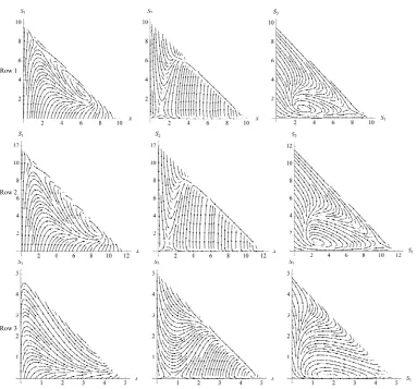
Numerical results using f given by (3) (noninteractive complementary), (4) (interactive complementary), and (5) (substitutable) using the parameter values given in Table 2 are illustrated in Figure1. In the figure, we can
ob-serve that substitutable nutrients lead to higher popula-tion densities than do complementary nutrients, which is not surprising. However, the differences in the densities from noninteractive and interactive nutrients are more surprising. When the nutrients are interactive, Rows 1 and 2 show that there can be a second (unstable) equi- librium population density. The stable population density is attained more quickly when the nutrients are interact- tive than when they are noninteractive. Finally, the stable
population density is generally higher when the nutrients are interactive than when they are noninteractive.
In fact, the population densities can be quite large as illustrated in Figure2. Consider the values listed in Row
2 of Table2 (corresponding to Row 2 of Figure 1). In Figure 2, we increase D (the washout rate) from D =
0.25 to D = 0.75 (row 1), D = 1.25 (row 2), and D = 1.75 (row 3). Observe that as D increases, interactive com-plementary nutrients lead to higher population densities than do noninteractive complementary nutrients. In fact, when the washout rate is sufficiently high, extinction occurs when the nutrients are noninteractive comple-mentary while stable persistence occurs when the nutri-
Row 1
Row 2
Row 3
[image:3.595.119.477.254.707.2]Row 4
Row 1
Row 2
[image:4.595.82.513.80.501.2]Row 3
Figure 2. Row 1: D = 0.75; Row 2: D = 1.25; Row 3: D = 1.75. Table 1. Descriptions of the constants in Equations (2)-(5).
S1(0), S2(0) Input concentration of the nutrients S1 and S2
D Dilution (washout) rate of chemostat m1, m2 Maximal growth rate of ith competitor
K1, K2 Michaelis-Menten (half-saturation) constants
y1, y2 Yield constants
f (S1, S2) Growth rate
Entes are interactive and complementary.
3. An Intermediate Metabolite
A particularly interesting situation occurs when one sub-stance degrades to a nutrient for the growth of an organ-ism. Specifically, Sanchez et al. [18], study the particular
situation in which phenol degrades to an intermediate metabolite that is then the primary nutrient for the organ-ism (bacterium Pseudomonas putida Q5). This situation is particularly interesting because a “harmful” substance degrades to a state in which it is a nutrient for the organ-ism under consideration that is growing in the chemostat, rendered harmless, and eliminated. To model this situa-tion, System (2) is adjusted to
0 1
1 1 1 1 2 1
1
2
2 1 1 2 2 2 2
1
2 2
d
, , 0 0
d d
, ,
d
d , 0 0,
d
S x
S S D f S S S
t y
S DS x f S S f S x S
t y
x f S D x x
t
0 0
(10)
[image:4.595.56.287.535.645.2]
1 1 2 1 1 21 1 1 1
, p n,
a b
m S S
f S S
K S K S
(11) where
2 2
11 1
S p p p e and
2 2
11 1
S n n n e
and f2 = a·S2 to data obtained from their study of
bacte-rium Pseudomonas putida Q5. With p = n = 1 and m1 =
m1m2 (Notation in Equations (3)-(5).) and f2 = a·S2, (11)
is the same as (4).
Although we cannot reduce System (10) to a single equation as with System (2), we can reduce it to a system of two equations. To do so, let
Then, and System (10) can rewritten as
0
1 1 2 .
S S S
x
D
0 22 1 1 2 2 2 2
1 2 2
d d
d , ,
d
d .
d
D t
S DS x f S S x S f S x
t y
x f S D x
t (12) Because the solution of is as
, in the limit as , System (12) is asymp-totic to the system
D
t 0
Dt Ce
t
0 22 1 1 2 2 2 2
1 2 2 d , , d d . d S x
DS f S S x S f S x
t y
x
f S D x
t
(13)
For the problem to be biologically meaningful, the feasi-ble region is
0
2 2 1 2
, 0, 0,
x S x S S S x
0 . (14) Assuming Monod kinetics, we now assume that f1
takes the form given by (11) and that n = p = 1 and that
2 2 2 2 2 2 2 .
f S m S K m S
The rest points of System (13) are E02
0,0 and potentially two interior rest points of the form
*
2 2
, I
E x DK m D ,
where
Evaluated at 02, the Jacobian has eigenvalues λ1,2 =
−D, so is always stable. E
2
0
If we eliminated S2 rather than S1, the limiting system
is E
0 0 11 1 1 1 1
1 0
2 1 1
d
, d
d d
S S S D x f S S S x
t y
x f S S x D x
t
(15)
with feasible region
0
1 1 1 1
, 0, 0,
x S x S S S x
0 . (16)
Again, assuming that f1 takes the form given by (11)
and that n = p = 1 and that f S2
2 m S2 2
K2S2
,we find that System (15) has rest points 1
0
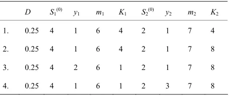
0 0, 1 [image:5.595.311.539.446.542.2]E S Table 2. Parameter values used for Figure 1.
D S1(0) y1 m1 K1 S2(0) y2 m2 K2
1. 0.25 4 1 6 4 2 1 7 4
2. 0.25 4 1 6 4 2 1 7 8
3. 0.25 4 2 6 1 2 1 7 8
4. 0.25 4 1 6 1 2 3 7 8
0 0 *2 2 1 2 1 2 1
0 0
1 2 1 2 2 1 1 1 2 1 1
2
2 2 2 0 0
2 2 1 2 1 2 1
0 0
2 1 2 1 2 1 2 2 1 1 1
0 0 0
1 2 1 1 2 1 1
2 2
2 0 2 2
2 1 2 1 2 1 1 1 2
2
2
2
b b a a
b b a
a
b b a
x D m K m m S D K S
D K K K m m K S D K K S y
D m K m m S D K S
K m D m D K K K m m S K S
D K K S S K S y
D m D K K K m K S y D m
1 2 1 22 1 1
b 1
K D m y
K m Dy
and potentially two interior rest points of the form
uated at obian has eigenvalues λ1,2 =
1 2
* *
1
, I
E x S , where and
the Jac Eval
−D 02
E , , so E02 is always stable.
Finally, if we had eliminated x rather than S or S, the limiting system is
01 1 2
1 1 1 1 2
1 0
2 1 1 2
2 1 1 2
1 0
2 2 1 1 2
, d
d
, d
S S S
S S D f S S
t y
S S S S
DS f S S
t y
f S S S S
(17)
with feasible region
0 1
dS
0
2 1 1 2
0,S 0,S S S 0 .
(18)
Using the same assumptions regarding f1 and
m
1, 2 1
S S S
f2 and
ade previously, the rest points of System (17) are
3
0 * *
0 1, 2 1 ,0
E S S S and potentially two interior rest points of the form
* *
1
, I
E x S E *
1, 2 2
I S DK m D , where
re 3 shows the behavior of Systems (13), (15),
and (17) using the parameter values in Figu Table 3. In all
three cases, the plots indicate that all solutions tend to
0
1 2 1
, , 0, ,0
x S S S as t . However, in the first
*2 1 2 1 2 1 1
0 0 0
2 1 2 1 2 1 1 2 1 2 2 1 1 1 2 1
2
0 0
2 2
2 1 2 1 2 1
0 0
2 1 2 1 2 1 2 2 1 1 1
0 0 0
1 2 1 1 2 1 1
2
2 0
2 1 2 1 2 1 1
1 2
2
2
b
b b a a
b b a
a
b b a
x
D m K D m y K m Dy
0 1
K m m S D K S D K K K m m K S D K K S y
K m m S D K S
K m D m D K K K m m S K S
D K K S S K S y
D m D K K K m K S
2 1 2
1
y
* 12 1 2 1 2 1 1
0 0 0
2 1 2 1 2 1 2 1 2 1 2 1 1 1
2
0 0
2 2
2 1 2 1 2 1
0 0 0 0 0
2 1 2 1 2 1 2 2 1 1 1 1 2 1 1 2 1 1
2 2
2 0 2
2 1 2 1 2 1 1 1
1 2
2
b
b b a
b b a a
b b a
S
D m K D m y K m Dy
K m m S D K S D m D K K K m K S y
K m m S D K S
K m D m D K K K m m S K S D K K S S K S y
D m D K K K m K S y
* 12 1 2 1 2 1 1
0 0 0
2 1 2 1 2 1 2 1 2 1 2 1 1 1
2
0 0
2 2
2 1 2 1 2 1
0 0 0 0 0
2 1 2 1 2 1 2 2 1 1 1 1 2 1 1 2 1 1
1 2 2
2 0 2
2 1 2 1 2 1 1 1
1 2
2
b
b b a
b b a a
b b a
S
D m K D m y K m Dy
K m m S D K S D m D K K K m K S y
K m m S D K S
K m D m D K K K m m S K S D K K S S K S y
D m D K K K m K S y
Row 1
Row 2
[image:7.595.102.498.80.454.2]Row 3
Figure 3. Modeling growth when the nutrient is an intermediate state of the substrate using the parameter values in Table 3.
Table 3. Parameter values used for Figure 3.
D S1(0) y1 m1 K1a K1b m2 K2
1. 0.5 2 1 3 2 2 1 1 2. 0.5 6 1 3 2 2 1 1 3. 0.5 8 1 3 2 2 1 1
two cases there are no interior rest points. While in the third, when is increased to 8, (3,4), (3,1), and (4,1), igenvalue of the Jacobian evaluated at the rest point is λ1
= −0.08
More interesting behavior of the systems is illustrated in Figu 4 where w use eter values in T le 4 he re lustr s t when (in t co
n-tration rate), m r m h ra ar in-c sed uil ium ates cur
al ee tuat s, t e is one u le rest t, , S1, S2) = (1.76, 7.24, 1), (1.54, 9.46, 1), and (0.260,
4.56, 0.143) as shown in Table5. However, in the first
two rows of Table 5, (x, S1, S2) = (6.23, 2.76, 1) and
(8.46, 2.54, 1) are stable spirals while in the third row, (x,
S1, S2) = (2.92, 1.93, 0.143) is an unstable spiral.
Thus, depending on the parameter values equilibrium states may be stable or unstable. Moreover, slight ad-justments to the parameter values might make a stable state unstable and vice-versa.
4. Conclusions
In this paper, we have formed a model of g h in a We have used numerical results to graphically illustrate
le
than do complement- ta
inte
mentary nutrients. It is possible that if the nutrients are
0 1
S
respectively, are degenerate rest points. For each, one chemostat with two interactive complementary nutrients. e
33 and the other is λ2 = 0.
re e the param ab
. T figu il ate hat 0 1
S (growt
pu nce of the subst
, eq 1
, o oc . 2
tes) e rea ibr st
In l thr si ion her nstab poin (x
rowt
differences in the behavior of systems modeling nonin- teractive comp mentary nutrients, interactive comple- mentary nutrients, and substitutable nutrients. Not sur- prisingly, we have illustrated that substitutable nutrients lead to higher population densities
Row 2
[image:8.595.108.491.80.437.2]Row 3 Row 1
Figure 4. Modeling growth when the nutrient is an intermediate state of the substrate using the parameter values in Table 4.
Table 4. Parameter values used for Figure 4.
D S1(0) y1 m1 K1a K1b m2 K2
interactive, the organism will attain a stable population density while if the nutrients are noninteractive, the or-ganism will become extinct. The simulations indicate that interactive complementary nutrients frequently lead to higher population densities than do noninteractive complementary nutrients. This agrees with the experi-mental results of Whang et al. [9] that show that com-plementary substrates (glucose and peptone) significantly increased hydrogen production by anaerobic hydrogen- producing bacteria.
A slight adjustment to the system leads to a completely different interpretation of the model in which the nutrient
the parameter values and slight adjustments to them can cause a stable state to become unstable and vice v This es with experi l res -chez et al. [18], which illustrated that slight ts
of the i ntr orre g
ma r e t rate
to 1 2) = , 0).
M a ks t u
carry out many of the calculations as well as generate the
1. 0.5 10 1 3 2 2 1 1
2. 0.5 12 1 3 2 2 1 1
[image:8.595.59.287.584.737.2]3. 0.25 5 1 8 2 2 2 1
Table 5. Rest points and eigenvalues of Jacobian for Figure 4.
Row x-S1 x-S2 S1-S2 Eigenvalues of Jacobian
(1.76,7.24) (1.76,1) (7.24,1) −0.359, 0.298
1 ±
0i
.54,9 .54, 1 − 0
2 8.46, .54,1 1.26142
.26
56 0.29143 ( 56,1.43) 0. −0.
(2.92, 0.0401 ±
(6:23, 2:76) (6.24,1) (2.76,1) −0.9830.85
(1 .46) (1 1) (9.46, ) 0.373, .311
2
(8.46, .54) ( 1) (2 ) −0. i ±
(0 0,
4. ) (0. 6, ) 4. 230, 224
3
(2.92,1.93) 0.143) (1.93,0.143) 0.919i
is an intermediate byproduct of the substrate. The simu-lations indicate the equilibrium states are very sensitive to
ersa. agre the menta ults of San adjustmen nlet conce ation (c spondin to 0
1
S ) had jo ffects on the
converges (xwashou, S, S (0, (when the limit as S0
t
e
1
a
figures a by email request t B
In future studies, w o exam
relationships (competition, pred ) are modeled nces s hes
re available from o Jim
the aut raselton.
hors sending an e hope t ine how com
ator-prey, and so petitive
forth under circumsta uch as t e.
REFERENCES
[1] S. R. Hansen and S. P. Hubbell, “Single Nutrient Micro-bial Competition: Agreement between Experimental and Theoretical Forecast Outcomes,” Science, Vol. 20, No. 4438, 1980, pp. 1491-1493.
http://dx.doi.org/10.1126/science.6767274
[2] H. L. Smith and P. Waltman, “The Theory of the Chemo-stat: Dynamics of Microbial Competition, Cambridge Studies in Mathematical Biology,” Cambridge University Press, Cambridge, 1995.
http://dx.doi.org/10.1017/CBO9780511530043
[3] C. P. L. Grady, Jr., G. T. Daigger and H. C. Lim, “Bio-logical Wastewater Treatment,” Second Edition, revised and expanded, Marcel Dekker, New York, 1999. [4] U. Lendenmann and T. Egli, “Kinetic Models for the
Growth of Escherichia Coli with Mixtures of Sugars Un-der Carbon-Limited Conditions,” Biotechnology and Bio-engineering, Vol. 59, No. 1, 1998, pp. 99-107.
http://dx.doi.org/10.1002/(SICI)1097-0290(19980705)59: 1<99::AID-BIT13>3.0.CO;2-Y
[5] P. G. Stroot, P. E. Saikaly and D. B. Oerther, “Dynamic Growth Rates of Microbial Populations in Activated Sludge Systems,” Journal of Environmental Engineering, Vol. 131, No. 12, 2005, pp. 1698-1705.
http://dx.doi.org/10.1061/(ASCE)0733-9372(2005)131:12 (1698)
[6]
edings o of Civil Engineers, New
[7] J. L. Sherwoo . Skeen and N. B.
19960905)51: W. Bae and B. E. Rittmann, “Effects of Electron Accep-tor and Electron Donor on Biodegradation of CC14 by Biofilms,” Environmental Engineering: Proce
the 1990 Specialty Conference, American Society f
York, 1990, pp. 390-395. d, J. N. Petersen, R. S
Valentine, “Effects of Nitrate and Acetate Availability on Chloroform Production during Carbon Tetrachloride De-struction,” Biotechnology and Bioengineering, Vol. 51, No. 5, 1996, pp. 551-557.
http://dx.doi.org/10.1002/(SICI)1097-0290( 5<551::AID-BIT7>3.0.CO;2-B
[8] D. V. Vayenas and S. Pavlou, “Coexistence of Three Microbial Populations Competing for Three COMPLE-MENTARY Nutrients in a Chemostat,” Mathematical Biosciences, Vol. 161, No. 1-2, 1999, pp. 1-13.
http://dx.doi.org/10.1016/S0025-5564(99)00040-1 [9] L.-M. Whang, C.-J. Hsiao and S.-S. Cheng, “A Dual-Sub-
strate Steady-State Model for Biological Hydrogen Pro-duction in an Anaerobic Hydrogen Fermentation
Proc-ess,” Biotechnology and Bioengineering, Vol. 95, No. 3, 2006, pp. 492-500. http://dx.doi.org/10.1002/bit.21041 [10] P. M. Bapat, S. Bhartiya, K. V. Venkatesh and P.
Wangi-kar, “Structured Kinetic Model to Represent the Utiliza-tion of Multiple Substrates in Complex Media During Rifamycin B Fermentation,” Biotechnology and Bioengi-neering, Vol. 93, No. 4, 2006, pp. 779-790.
http://dx.doi.org/10.1002/bit.20767
[11] P. Champagne, P. J. Van Geel and W. J. Parker, “A Pro-posed Transient Model for Cometabolism in Ciofilm Sys-tems,” Biotechnology and Bioengineering, Vol. 60, No. 5, 1998, pp. 541-550.
http://dx.doi.org/10.1002/(SICI)1097-0290(19981205)60: 5<541::AID-BIT4>3.0.CO;2-Q
[12] W. Bae and B. E. Rittmann, “A Structured Model of Dual-Limitation Kinetics,” Biotechnology and Bioengi-neering, Vol. 49, No. 6, 1996, pp. 683-689.
http://dx.doi.org/10.1002/(SICI)1097-0290(19960320)49: 6<683::AID-BIT10>3.3.CO;2-E
[13] M. M. Ballyk and G. S. K. Wolkowicz, “Exploitive Com-petition in the Chemostat for Two Perfectly Substitutable Resources,” Mathematical Biosciences, Vol. 118, No. 2, 1993, pp. 127-180.
http://dx.doi.org/10.1016/0025-5564(93)90050-K [14] G. J. Butler and G. S. K. Wolkowicz, “Exploitive
Com-petition in a Chemostat for Two Complementary, and Possible Inhibitory, Resources,” Mathematical Biosci-ences, Vol. 83, No. 1, 1987, pp. 1-48.
http://dx.doi.org/10.1016/0025-5564(87)90002-2
[15] S-B. Hsu, K-S. Cheng and S. P. Hubbell, “Exploitive Competition for Two Complementary Nutrients in Con-tinuous Cultures,” SIAM Journal on Applied Mathematics, Vol. 41, No. 3, 1981, pp. 422-444.
http://dx.doi.org/10.1137/0141036
[16] S.-B. Hsu and Y.-H. Tzeng, “Plasmid-Bearing, Plas-mid-Free Organisms Competing for Two Complementary Nutrients in a Chemostat,” Mathematical Biosciences, Vol. 179, No. 2, 2002, pp. 183-206.
http://dx.doi.org/10.1016/S0025-5564(02)00105-0 [17] H. R. Thieme, “Convergence Results and a Poincaré-
Bendixson Trichotomy for Asymptotically Autonomous Differential Equations,” Journal of Mathematical Biology, Vol. 30, No. 7, 1992, pp. 755-763.
http://dx.doi.org/10.1007/BF00173267
[18] J. L. Garcia-Sanchez, B. Kamp, K. A. Onysko, H. Bud-man and C. W. Robinson, “Double Inhibition Model for Degradation of Phenol by Pseudomonas Putida Q5,” Bio-technology and Bioengineering, Vol. 60, No. 5, 1998, pp. 560-567.