Spectral Analysis Informs the Proper Frequency in the Sampling of Financial Time Series Data

Munich Personal RePEc Archive

Spectral Analysis Informs the Proper

Frequency in the Sampling of Financial

Time Series Data

Taufemback, Cleiton and Da Silva, Sergio

2011

Online at

https://mpra.ub.uni-muenchen.de/28720/

Spectral analysis informs the proper frequency in the

sampling of financial time series data

Cleiton Taufemback

Sergio Da Silva

Graduate Program in Economics, Federal University of Santa Catarina, Florianopolis SC 88049-970, Brazil

Abstract. Applied econometricians tend to show a long neglect for the proper frequency to be considered while sampling the time series data. The present study shows how spectral analysis can be usefully employed to fix this problem. The case is illustrated with ultra-high-frequency data and daily prices of four selected stocks listed on the Sao Paulo stock exchange.

1. Introduction

How often to sample a continuous time series? In the presence of market microstructure, for example, Ait-Sahalia et al. [1] suggest the rule of thumb of sampling “as often as possible.” Here, we propose a precise method to find the proper frequency. It is unusual for applied econometricians to analyze a time series from the perspective of the frequency domain, that is, they usually do not consider the spectral analysis of the frequency. Here, the first concept highlighted is the Nyquist-Shannon sampling theorem presented in 1949 in the pioneering work of Shannon [2]. This theorem has given rise to the then new area of information theory.

According to the theorem, for a sampled signal to convey all the original information it is necessary for the signal to be sampled at a rate which is at least two times larger than the highest frequency in the spectrum [3, 4]. If a function ( )f t

contains no frequencies higher than W Hz, it is completely determined by giving its ordinates at a series of points spaced ½ seconds W apart [2].

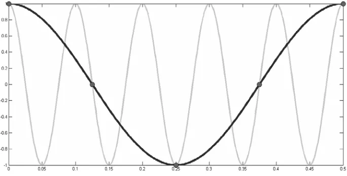
Thus, undersampling may introduce errors in the signal. One standard example is to consider two distinct frequencies that are mistakenly taken as identical due to undersampling [5]. Let

cos(2x_t = π ft t∆ ), (1)

where ∆t is the sampling time period. Then, for * 1

t

f = −_∆ f , where

(

)

f ∈ _∆ , one has

*

cos(2 ) t

x = πf t t∆

(

)

(

)

=cos 2π _∆−f t t∆

( )

(

)

=cos 2πt +cos −2πft t∆

(

)

= +1 cos 2πft t∆ . (2)

Aliasing has been systematically neglected by applied econometricians despite the (scant) warnings of a few theoretical econometricians. Granger and Newbold [6] provide a theoretical example where data containing weekly cycles sampled at a monthly frequency generate a spurious peak in the spectrum. Ashley and Dwyer in an unpublished working paper [7] give another example of aliasing. Here, an AR(6) time series is generated and then resampled at different frequencies to show how poorly sampled regressions in the series are prone to errors of coefficient estimation.

In a startling contrast to applied econometricians, analyses of the frequency domain are widespread in well developed areas, such as biology, astrophysics, engineering, and telecommunications. Spectral analysis is routinely used in all applications where either oscillatory properties or pattern recurrence are present in a signal.

The Fourier transform is the main toolkit employed to learn the characteristics of a series in the frequency domain. It works like regressing a series to a sum of sinusoids. As a result, the coefficient values of a given frequency represent the signal amplitude of the frequency. A continuous Fourier transform ℑ takes the form:

( )w f t e( ) iwtdt ∞

− −∞

ℑ =

∫

where w=2πf .

Another key ingredient of spectral analysis is the power spectral density function, which represents the amount of energy for each frequency analyzed in a stochastic process. It is also the representation in the frequency domain of the autocorrelation function, through the Fourier transform. A continuous power spectral density function is given by:

2

*

1 ( ) ( )

( ) ( )

2 2

iwt w w

w f t e dt

π π

∞

− −∞

 _{ ℑ ℑ}

 _

Φ =_{ } =



∫

The present study demonstrates how neglecting aliasing could be harmful in the context of sampling financial prices. Samples of ultra-high-frequency historical price time series of four selected stocks listed on the Sao Paulo stock exchange (Bovespa, for short) were taken. The study demonstrated how sampling on a daily basis, using the tick-by-tick data as the raw data, violates the Nyquist-Shannon sampling theorem.

The rest of the present article is organized as follows: section 2 presents data and the methods used, section 3 shows the results, and section 4 concludes the study.

2. Data and methods

The ultra-high-frequency price time series data considered are for the stocks of Ambev PN (AMBV4; 514,302 observations), Sid Nacional On (CSNA3; 1,359,702 observations), Petrobras PN (PETR4; 5,381,081 observations), and Vale PNA N1 (VALE5; 5,220,472 observations), which are listed on the Bovespa. The sample period ranged from 11:00 am on January, 2 2007 to 06:00 pm on December, 30 2008. The four stocks have been selected on the basis of the largest trade volume and foreign visibility.

Using interpolation of the missing observations, interpreting them as zero, or keeping the last measured observation as constant until the next one appears are all poor alternatives [8]. Here, it would be preferable to resort to the Lomb-Scargle method [9, 10], which makes use of the series of sines and cosines and takes only the observations sampled, with no need of interpolation. The Lomb-Scargle method can also be used to evaluate any previous interpolation, signal resample, and autoregression conditional duration [11]. However, this method is not free of problems, especially when ultra high frequency is involved [12, 13].

As a result, the present work considers the Bayesian spectrum estimation [14], which fits well for analyzing the time evolution of the frequency spectrum of commonly nonstationary financial data. This method does not rely on the need for the series to be stationary. Further, time windows have also been dismissed. It jointly estimates the newly generated data observation by updating the coefficient values using a nonstationary Kalman filter.

However, unlike the Lomb-Scargle method, the Bayesian spectrum estimation is not equipped with a straightforward way of reckoning the significance of an estimated coefficient. To fix this problem, a large range of the spectrum was considered by taking many coefficient values. In addition, a t test was also performed to learn whether the coefficient value c_i was distinguishable from the mean c . For each coefficient value the null hypothesis (H₀) was tested against the alternative (H₁):

0: 1.5i

H c < c

1: 1.5i

H c ≥ c (5)

where the value 1.5 was parsimoniously chosen on a trial and error basis.

As the Bayesian spectrum estimation is quite sensitive to the chosen inputs, maximum frequency and interval number, it is appropriate to use a high value for the frequency and then reduce this value until a proper value is met.

Further, it is necessary to inform the moment when each observation is sampled as the times series used are unevenly spaced. Figure 2 demonstrates how to tackle this issue. Here, an observation is adjusted to differ from the precedent observation in seconds. Thus, in this procedure periods without activity, such as weekends, holidays and closing hours, have been computed. This reinforces the significance of the coefficient for the continuous state, 0 Hz. Thus, the estimate is made even more parsimonious for the high frequency data used in the method.

3. Results

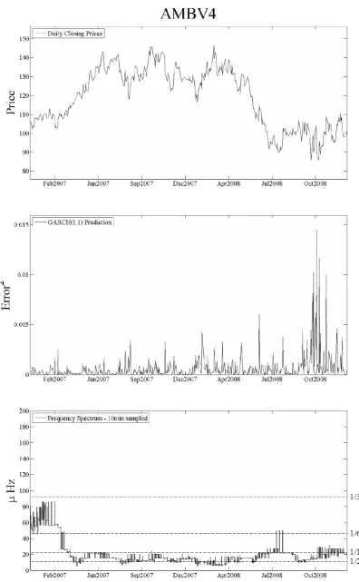
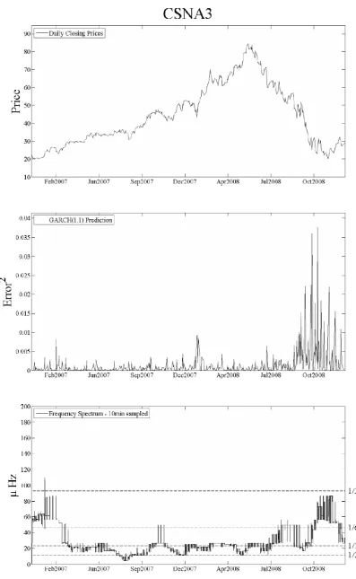
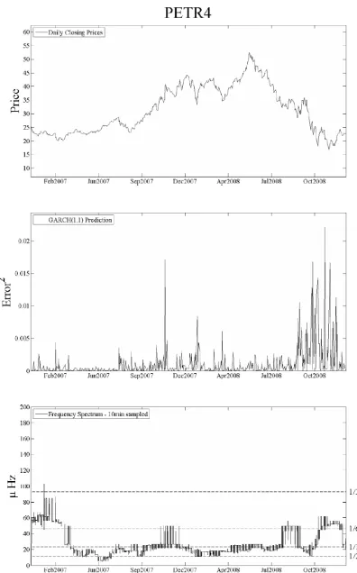
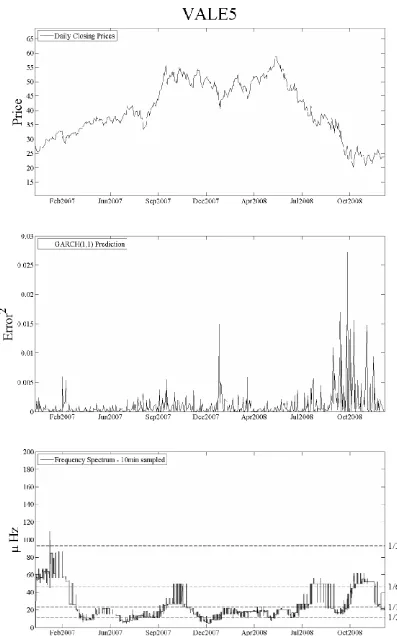
Using the ultra-high-frequency raw data, it was observed that the four stock prices never overshot frequencies higher than 277.8µHz. This corresponded to a period of one hour. Based on the obtained results and the fact that the series were not regular in time, the original raw series were resampled and samples were taken at an interval of 10 minutes each. It was observed that this procedure was well above the recommended Nyquist-Shannon rate. The new series were then reestimated to make it possible to contrast the significant frequencies with the daily series. Figures 3-6 show the obtained results.

be sampled at least at the frequency of 185.2µHz, which corresponds to a period of one and a half hours.

As an exercise, a GARCH(1,1) process was considered for forecasting a day ahead. Figures 3-6 show the results in terms of quadratic errors. The error series show large values when the frequency spectrum is high (aliasing), as well as when there is a significant change in the values of the last frequency, which can be attributed to financial volatility.

In the field of telecommunications low-pass filters are used as a common solution for the presence of undesirable high frequencies. These filters remove the influence of the high frequencies while keeping the desirable signal, which is then resampled at a more convenient rate. However, anti-aliasing filters are likely to bring more costs than benefits when the financial series are at stake [15].

4. Conclusion

Spectral analysis is widespread in well developed areas, such as biology, astrophysics, engineering, and telecommunications. It is mainly used in applications where either oscillatory properties or pattern recurrence are present in a signal. However, applied econometricians tend to neglect the proper frequency to be considered while sampling the time series data. The present study shows how spectral analysis can be usefully employed to fix this problem. The case is illustrated with ultra-high-frequency data and the daily prices of the four selected stocks listed on the Sao Paulo stock exchange.

The study demonstrated how neglecting aliasing by resampling on a daily basis, using the tick-by-tick data as the raw data, violates the Nyquist-Shannon sampling theorem. In general, the four stock price series display frequencies higher than 11.6µHz

References

[1] Y. Ait-Sahalia, P.A. Mykland, L. Zhang, How often to sample a continuous-time process in the presence of market microstructure noise?, Review of Financial Studies 18 (2005) 351.

[2] C.E. Shannon, Communication in the presence of noise, Proceedings of the Institute of Radio Engineers 37 (1949) 10.

[3] S. Haykin, Communication Systems, 4th edition, New York, John Wiley & Sons, Inc., 2000.

[4] T.S. Rappaport, Wireless Communications: Principles and Practice, 2nd edition, Upper Saddle River, Prentice Hall, 2002.

[5] P. Bloomeld, Fourier Analysis of Time Series: An Introduction, 2nd edition, John Wiley & Sons, Inc., 2000.

[6] C. Granger, P. Newbold, Forecasting Economic Time Series, New York, Academic Press, 1977.

[7] R.A. Ashley, J.G.P. Dwyer, Time domain aliasing and nonlinear modelling, Virginia Tech working paper, 1998.

[8] W.H. Press, B.P. Flannery, S.A. Teukolsky, W.T. Vetterling, Numerical Recipes in FORTRAN 77: The Art of Scientific Computing, 2nd edition, New York, Cambridge University Press, 1992.

[9] N.R. Lomb, Least-squares frequency analysis of unequally spaced data, Astrophysics and Space Science 39 (1976) 447.

[10] J.D. Scargle, Studies in astronomical time series analysis. II – Statistical aspects of spectral analysis of unevenly spaced data, Astrophysical Journal 263 (1982) 835.

[11] I. Giampaoli, W.L. Ng, N. Constantinou, Analysis of ultra-high-frequency financial data using advanced Fourier transforms, Finance Research Letters 6 (2009) 47.

[12] G.L. Bretthorst, Generalizing the Lomb-Scargle periodogram, American Institute of Physics Conference Proceedings 568 (2001) 241.

[13] M. Zechmeister, M. Kurster, The generalised Lomb-Scargle periodogram. A new formalism for the floating-mean and Keplerian periodograms, Astronomy & Astrophysics 496 (2009) 577.

[14] Y. Qi, T.P. Minka, R.W. Picard, Bayesian spectrum estimation of unevenly sampled nonstationary data, ICASSP 02 IEEE International Conferences 2 (2002) 1473.

Figure 1. The aliasing phenomenon: A sinusoid of frequency equals to 10Hz. If it is sampled at 8Hz it could be mistakenly confused with a sinusoid of 2Hz.

Figure 6. Price series of Vale PNA N1: Top: daily closing prices. Middle: GARCH(1,1) prediction series. Bottom: 10-minute sampled frequency spectrum.