Behind the North South divide: A decomposition analysis

Munich Personal RePEc Archive

Behind the North-South divide: A

decomposition analysis

Vizer, David

The University of Aberdeen

12 January 2011

Online at

https://mpra.ub.uni-muenchen.de/28364/

Behind the North-South divide

– A Decomposition Analysis

David Vizer

January 2011

JEL: C13 C20 C30 J21 J24 J31

Keywords: North-South divide, regional wage gap, Oaxaca decomposition

9670 words

Table of contents

1. Introduction 6

2. Literature review 8

3. Methods 12

3.1 Wage equation 13

3.2 Sample selection 14

3.3 Oaxaca decomposition 15

3.4 Identification issue 19

3.5 Juhn, Murphy and Pierce (1991) decomposition 20

3.6 Limitations of the Oaxaca-type analyses 21

3.7 North-South divide coefficient 22

4. Data and Estimation 23

4.1 Variable and model specification 23

4.2 The sample 25

4.3 The wage gap 27

4.4 Insights from the year-by-year OLS results 30

4.5 Oaxaca decomposition results 33

4.6 North-South divide coefficient 38

4.7 JMP decomposition results 39

5. Conclusion 45

References 46

Summary

The paper applies modified Oaxaca-type analyses on the eighteen available waves of the British Household Panel Survey to decompose the wage gap among full time employees from either side of the North-South divide and identify its components that can be attributed to measurable worker- and labour market characteristics, and the part due to differences in the returns to these endowments. Further, by applying Juhn, Murphy and Pierce’s (1991) methodology, it is analysed, how changes in these underlying factors could explain the one quarter decline in the wage gap over the 1991 – 2009 period.

Acknowledgements

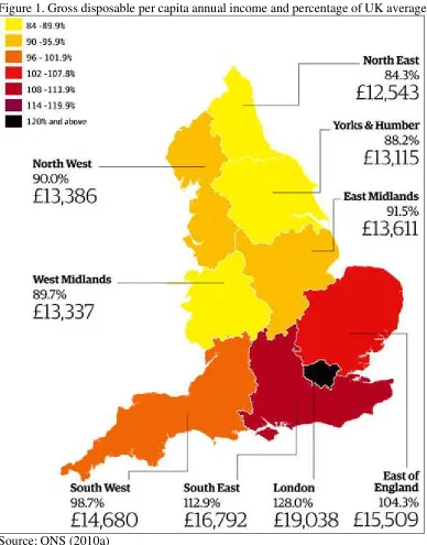
Figure 1. Gross disposable per capita annual income and percentage of UK average

Source: ONS (2010a)

“The north-south divide is no longer a vague idea […] We have enough information on life chances, health and wealth to say where the line lies and what is happening to it.”

1. Introduction

In its most recent bulletin, the Office for National Statistics (2010a) – inadvertently – maps the North-South divide by its favourite measure: average per capita labour and non-labour income after taxes, housing costs and benefit receipts. The same bulletin reports that while in 1995 the most and least affluent regions – London and Yorkshire & Humber – were 20% above and 9% below the national average, by 2009 the gap widened to 28% and 12% respectively, amounting to an over £10,000 difference in annual incomes. All major newspapers – broadsheet and tabloid alike – cited the figures, just as they did in the past forty years with any other socio-economic data that pointed to the dichotomy between North and South. As a result, few would question the existence of the divide, yet the emergence of the phenomenon owes much more to the populist press than to any robust economic analysis.

The Severn – Wash line1 has been separating income and wage levels, employment opportunities, health conditions, life expectancy, educational attainment and house prices for a century (Doran 2004, Baker and Billinge 2004). However, only after the 1970s’ industrial restructuring, which resulted in record levels of cross-regional income and unemployment disparities (Hudson 1989, Armstrong and Taylor 1987), did the North-South divide become widely discussed. While there is hardly any week without being mentioned in the national press, there has been markedly little research attempting to evaluate the true extent of such a divide in any robust way, yet alone in a dynamic setting. This paper adds to the existing literature by performing static and dynamic decomposition

1

analyses on eighteen years’ (1991-2009) panel data to investigate the forces behind England’s South average wage gap – the most significant gap within the North-South divide context1 – and the change of their magnitudes over time. The paper adopts novel econometric techniques and proposes a unique three-fold specification to correct for a number of shortcomings of the original Oaxaca method, such as getting biased estimates on the relative size of the endowment and coefficient effects’ individual components caused by both the excluded categorical variables and the inevitable choice of an implicit non-discriminatory norm. The study seeks to identify whether there is an adjusted wage gap – a residual left over after controlling for measurable regional worker and labour market characteristics –, and along what dimensions is the gap changing between 1991 and 2009 both in terms of endowments and the returns to these attributes; as only such a residual could be sensibly called the North-South divide, meaning the gap between wages of comparable workers. By estimating the magnitude of the unexplainable part of the pay gap at different inter-decile ranges in the wage distribution, the paper will conclude by proposing a method to evaluate the robustness of its findings across the whole wage distribution.

1

2. Literature review

Neoclassical theory suggests that regional income inequality may arise due to temporary demand/supply disequilibrium (Blackaby and Manning 1990); compensating differentials for job characteristics, regional price levels, unemployment or crowding (Rosen 1986, Bergmann 1971); or caused by institutions, such as collective bargaining, efficiency wages or employment legislation, through their effects on labour market flexibility. The theory suggests that after controlling for all such determinants, and provided that sufficient time is given1, factor prices will equalize for comparable workers and the resulting wages should be inter-regionally invariant. Competing theories, on the other hand, such as the Big Push model by Rosenstein-Rodan (1943) explain regional income inequalities from a very different perspective. These propose that regional disparities may not decrease over time as more prosperous regions build on the scale-economies and knowledge spill-overs of their concentrating industries (Lucas 1988) leading to the emergence of clusters of economic miracles (Porter 2000) which, reinforced by a unidirectional movement of workers, could initiate vicious circles of self-reinforcing relative decline in the less affluent regions. It is very difficult to model wage determination by such forces in micro-studies, therefore most analyses build on the neoclassical model and leave these effects to the intercept.

The study of income dispersion attracted substantial interest following a significant rise in earnings inequality in most OECD countries from 1978 onwards both between and within various groups of workers (see Katz and Autor 1999 for a survey). Most studies trying to explain the strong positive correlation between income percentile rank and real increases in earnings attributed the phenomenon to growing returns to labour market skills, most

1

importantly to education and experience. Explanations included demand and supply shifts (Freeman and Katz 1994), the growing international trade (Borjas and Ramey 1995) as well as institutional factors (Nickel and Layard 1998). It has been observed that real earnings of skilled workers kept rising markedly even though their supply increased at the same time. The seemingly paradoxical relationship was reconciled by Katz and Murphy (1992) who suggested that demand shifts, driven by the increase in skilled workers’ productivity, must have been higher than the downward pressure on wages caused by the growing proportion of such workers. Machin (1995) and Autor et al. (1998) argued that the rise in skilled workers’ productivity was induced by a skill-biased technological change, which can also explain why real earnings of unskilled workers remained relatively stagnant for long periods of time. Not only had the so-called skill upgrade caused a drop in demand for the low skilled, but growing international trade allowed the substitution of these workers’ labour for cheaper imports, while declining unions and industrial restructuring further worsened their position by forcing the unskilled into sectors with low-average high-variance wage distribution. Several studies have suggested that bi-directional feedback effect mechanisms may aggravate pay differences over time, and also across regions, either through the well-established link between family income and educational attainment (Machin and Vignoles 2004), or through the industry structure affecting regional development in an unbalanced fashion by cumulatively distorting the inter-regional skill distribution (Chen et al. 2010).

North and South are far from being that homogenous as indicated by the concept of the North-South divide, and therefore no analysis at this aggregation would be meaningful. Also, by witnessing the record increases in within-group inequalities, influential writers like Shorrocks (1984), Jenkins (1994) or DiNardo et al. (1996) advocated the study of income inequalities across the whole income distribution, as it would convey more information than analysing averages1. The third reason why the study of the North-South divide might have been neglected could be due to American findings on the US North-South divide. During the 1960s and 1970s numerous papers using pre-Mincerian income models demonstrated the existence of the divide by showing that a large part of the North-South income gap cannot be explained by measurable differences between the regions (Scully 1969). When subsequent studies re-performed these estimations applying more sophisticated modelling and Oaxaca-type decomposition techniques, they all found that after taking worker characteristics, labour market differences and regional price levels into account, the remaining North-South income gap is no longer statistically significant (Sahling and Smith 1983).

The Oaxaca (1973) - Blinder (1973) approach was originally devised to calculate Becker’s (1971) discrimination coefficient and to analyse the gender pay gap in a meaningful way after controlling for observable differences (see Olsen et al 2009 for a UK update). The technique became the predominant tool in analyses of pay differentials aiming to identify the underlying sources of such disparities by quantifying the individual effects of the distribution of worker and labour market characteristics and their different returns on the pay gap. Several augmentations have been proposed over the years making it possible to

1 _{While not disagreeing with the proponents of studies of the second moment of income variance, it has to be}

decompose over-time changes in differentials (Juhn, Murphy and Pierce 1991); gaps between inter-quantile ranges or at specific percentile points (Makepeace et al. 1999, Buchinsky 1994, Machado and Mata 2005); as well as to analyse measures of distributions instead of mean-differences (Yun 2006). The method had a huge influence on micro analyses, and is even featured in court hearings.

The extensive search on EconLit and RePEc revealed only two papers that performed an Oaxaca-type decomposition analysis on England’s North-South income differential, of which none applied the over-time extension. Blackaby and Manning (1990) by analysing a 1975 and a 1982 dataset, found that only half of 1975’s approximately 6% annual income gap could be explained by the more favourable occupational, industrial and educational structure of the South, and only a third of 1982’s similar magnitude monthly income differential could be attributed to superior Southern endowments. Their results “only partly support the notion of a North-South divide”, however they suggest: “much may be learned by combining a sequence of cross-section data sets over time” (p524). Blackaby and Murphy (1995) by performing the same analysis on a 1983 income data, draw a similar conclusion by suggesting that the 2.4% income gap residual, remaining after endowments are controlled for, is not large enough to be inconsistent with neoclassical theory.

3. Methods

While the stark contrast between Southern and Northern incomes is visible on the map, it is not so obvious whether Southern workers earn more because there is a North-South divide per se, or because on average Southern workers have more favourable characteristics, or because these characteristics are rewarded more in the Southern labour market. The paper is going to decompose the wage gap to these distinct components to measure their relative contribution year-by-year over the period, and also – and more importantly from a policy perspective – it will decompose the over-time change in the wage gap to the underlying

actually underestimates discrimination as real discrimination starts earlier than employment, therefore using it with wage equations from a self-selected sample is insufficient to determine the true extent of the concern. On a similar note – even emphasised by Oaxaca (2007) –, if one could control for all variation in the wages, then the differential treatment, defined as the residual, could be completely eliminated. In the context of the North-South divide, this limitation must be addressed. By controlling for industry structure it is implicitly assumed that the different regional sectoral-mix is entirely explainable by workers’ voluntary choices, arriving to spurious findings which explain the wage gap by – say – Northern workers’ reluctance to work in finance. Although controlling for it, differences in the industry-mix will not be discussed as part of the endowment gap, as industrial crowding or segregation into lower paid industries are strongly influenced by a given industry structure, making it a possible source of the differential treatment effect.

3.1 Wage equation

The Oaxaca method works by measuring differences between regressor means and their coefficients after estimating a pair of earnings equations. As real world wage determination cannot be directly observed, it will be modelled as a stochastic process separately for Northern (N) and Southern (S) workers year-by-year, assuming that the wage (w) is determined by j number of worker and labour market characteristics:

N i N j N i N N i S i S j S i S S i u X w u X w           0 0 N S N i N i ,... 1 , ,... 1 ,   ) 2 ( ) 1 ( E E

gender, occupation or industry-mix, _j is a column vector of the parameters reflecting the

marginal returns to each wage determinant, ₀ is the intercept, while u is a random error

term with expected value of zero allowing for the effect of natural ability or luck.

3.2 Sample selection

As the dependent variable is not observed for individuals who cannot get an offer above their reservation wage, the regression would not be based on a random sample but on a censored, self-selected one. If there is a systematic relation between some of the wage determinants and individuals’ probability to work with these characteristics, the estimated coefficients in the wage equation would become inconsistent, as the error terms of the wage equation and the participation function fitted on individuals’ probability to work would correlate. Due to the comparatively higher labour force participation of male workers such bias is not assumed to significantly affect their wage determination. Following Heckman (1976, 1979) and Wooldridge (2002) to correct sample selection bias, the probability that a

woman will self-select and makes her wage observable (I_i 1) is estimated from the entire

sample, by modelling it as a function of Z_i, a vector of characteristics affecting

participation only (S1):









Pr I_i   Z_i _i   Z_i _i (S1)









i I X u I X

w | 1 ₀    | 1 ₀     (S2)

Where

 

 

_{ }

    

ˆ ˆ

i i i

i

Z Z Z

 

In the corrected wage equation (S2),  is the standard deviation of u;  is the correlation

between  and u;  is a new error term with expected value of zero, and  is the ratio of

the density function of the standard normal distribution to the cumulative normal distribution function, reflecting the estimated probability that a woman with specific characteristics mix will self-select to work. Including it will control for the non-random nature of self-selection, therefore the pooled-gender OLS will give consistent estimates on the parameter vector.

3.3 Oaxaca decomposition

Following the estimation of the wage function-pairs – and provided that the null hypothesis of no systematic difference between Northern and Southern coefficient vectors can be rejected – it is possible to break down the wage gap into an endowment effect (E), a part due to characteristic-differences between the representative Northern and Southern workers, and into a coefficient effect (C), a part due to differences in the returns to these endowments. The latter term, which also includes the differences between the intercepts, identifies the residual wage gap after measurable variation in the mean endowments has been controlled for, or in other words, the adjusted North-South divide.

counterparts in the North are underpaid – an assumption adopted by most studies of its kind despite of a major flaw in its formulation.













 





w jN N

S j N S S

j N S N

S    ˆ  ˆ ˆ  ˆ ˆ  

0 0

) 1 (O

As Jones and Kelley (1984) argue, weighting the coefficient gap by the less advantaged group’s endowment, as in (O1), is appropriate only if the policy attempts to close the gap by decreasing the more advantaged group’s endowment levels. Clearly, there are not many contexts where this would be the case. To address the specification issue, an alternative form (O2) has been suggested which, however, by allowing its coefficient gap to be tested at the Southern endowment vector, effectively forces its endowment term to be weighted by the Northern returns to wage determinants. Such a treatment creates an implicit assumption that Northern workers are paid fairly while their Southern counterparts receive unduly high

compensation – an assumption somewhat difficult to justify, which may explain why, despite its more sensible treatment of the coefficient effect, specification (O2) remains seldom used, and the few authors who feature it, do so only to demonstrate the robustness of their (O1) results.













 





w

wS  N  S  N ˆ_jN  ˆ₀S ˆ₀N  ˆS_j ˆ_jN S   (O2)

Oaxaca and Ransom (1988) point out that while both specifications will identify the most important components of the wage gap, the estimates of their relative contributions will be dependent on the chosen non-discriminatory norm, or in other words: the weighting of the endowment effect. They attempt to address the theoretical difficulty to select one reference over its alternative by proposing a generalised specification (O3) where by including both

offer the construction of an infinite number of non-discriminatory norms anywhere in-between the vectors of the North and the South including the two extremes, where  1 would form (O1), while equation (O2) could be given by setting  0. In the same framework, Cotton (1988) suggests averaging the vectors ( 0.5), while Reimers (1983) recommends making  equal to the relative population size of the corresponding region.

















w

wS  N  S  N S   N  S N  S  N  

) 1 ( ˆ ˆ ˆ

) 1 ( ˆ

1

) 3 (O

Others, like Neumark (1988) who used the coefficient vector from the two groups’ pooled

regression as the non-discriminatory reference (ˆ*), suggest that such a vector does not

have to be constructed from the analysed groups’ coefficients, it can be any external references, such as a third region’s vector, as in (O4).





















w

wS  N  S  N ˆ*  ˆS ˆ* S  ˆ*ˆN N   (O4)

Unfortunately, so far none of the specifications offered a definitive solution to the sensitivity of the relative size of the endowment effect to the chosen non-discriminatory reference. Another – very closely related – problem with all two-fold specifications is that they do not permit weighting the effects by the same group’s coefficient and average endowment vectors. In the current context it is not only reasonable to multiply the coefficient gap by the Southern endowments due to the direction of the policy, which aims to adjust Northern human capital (and even industrial) composition to Southern levels, but to use Southern coefficients also to evaluate the relative importance of inter-regional differences in the wage determinants – not offered by any previous arrangements. It can

reasonably be assumed that returns to wage determinants are negative and concave functions of their supply conditions. If the lower Northern supply of favourable wage determinants, like degree-level qualification, makes Northern wage premia relatively higher for these characteristics, extrapolating Northern endowments to Southern levels by using the North’s coefficients will inevitably overestimate the size of the endowment effect and the possible decrease in the wage gap upon successful convergence in the endowment levels. Even with the presence of the widely reported rise in skills premia, this non-linearity can be best approximated in a linear model by evaluating the relative size of the endowment gap using Southern coefficients.

To satisfy both requirements the reverse1of Jann’s (2008) three-fold specification (O5) will be adopted by using the Southern coefficient and endowment vectors to weight the endowment and coefficient gaps respectively and by specifying an interaction term (CE) in order to separately identify the primary components’ pure effects. With some manipulation, it is easy to see that the reason why the relative size of the effects was always dependent on the chosen non-discriminatory norm, is that in all previous two-fold specifications the (CE) component, which picks up the effect of the interaction by the endowment and coefficient gaps, was deducted from either the endowment (O1) or the coefficient effect (O2) depending on the chosen reference group. By stating the (usually opposite signed) interaction term separately, the true magnitude of the pure effect, of which it is grouped to, can be estimated.

















w

wS  N  S  N ˆS  ˆS ˆN S  S  N ˆS ˆN    (O5)

1

3.4 Identification issue

bears each characteristic from every sets, and therefore normalised in the sense that it will not pick up the differential return to any one category.

3.5 Juhn, Murphy and Pierce (1991) decomposition

While the static Oaxaca analysis at any one point in time can examine the existence of the adjusted North-South wage gap, the results may not be easily interpretable from a policy perspective, as – due to four different over-time forces – the method is incapable of telling how much change in the overall wage gap could be predicted by over-time changes in the underlying factors. If the wage gap is found to decrease over time, it could be caused by an improving relative skill-mix in the North, or by a deteriorating relative skill-mix in the South, or it may be explained by falling relative returns to wage determinants in the South, or by rising relative returns in the North. From a policy perspective the implication of the different effects could not be more different, therefore any meaningful decomposition must be capable of identifying these distinct forces. The traditional Oaxaca decomposition cannot fulfil this requirement, as it divides the wage gap into endowment and coefficient effects, which are both weighted differences, and therefore one cannot be sure whether an over-time change in the – say – endowment effect was caused by an actual change in the relative endowments, by a change in the relative weights, or by both.

wage gap as weights for their counterpart terms (second terms in J2 and J3).



 





 









 











X X

X X

X X

E ₂₀₀₉  ₁₉₉₁  ₂₀₀₉  ₁₉₉₁ ₂₀₀₉  ₁₉₉₁  ₁₉₉₁ ₂₀₀₉ ₁₉₉₁

 (J2)



 









 











X X

X

C ₂₀₀₉ ₂₀₀₉ ₁₉₉₁  ₂₀₀₉ ₁₉₉₁  ₂₀₀₉  ₁₉₉₁ ₁₉₉₁ ₁₉₉₁

 (J3)

3.6 Limitations of the Oaxaca-type analyses

over-time analysis on a panel dataset. Future research will have to try bridging the theoretical gap between the analyses of first and second moments of wage inequality, as even if one could measure all wage determinants and specify the ultimate model, coefficients estimated at the mean may not adequately explain associations across the whole distribution.

3.7 North-South divide coefficient

To address some of these limitations, and to suggest a possible test for the applicability of the estimates at different points of the wage distribution, analogously to Becker’s (1971) discrimination coefficient, a North-South divide coefficient (C1) will be constructed.









exp  

 N

d S d N d

X

C   (C1)

4. Data and Estimation

For any over-time study, longitudinal surveys are the datasets of choice for being consistent in the measurement of key variables, and for helping to reduce the potential unobserved heterogeneity bias between the years by tracking the same individuals over time. The analysis draws from the available eighteen waves (1991 – 2009) of the nationally representative British Household Panel Survey (University of Essex 2010, BHPS thereon). The data includes information on 10,000 individuals’ human capital, earnings, occupation, industry and social indicators. Even though its individual response rate was 74% at the first wave, the stratified design ensured that it remained representative. The sample is unbalanced due to attrition, but respondents’ new family members are entered in the survey and are also considered in this analysis. The selected sample is restricted to 16 – 691 years old full-time employees (>30 hours a week) from England resulting in 3,500 observations per year, 60,000 in total. Models are estimated in Stata10.0 and Microsoft Excel registered to the University of Aberdeen. The top 0.1% of earners with incomes over £150,000 per annum was excluded, such as rows of observations with missing information in any of the variables2. Additional algorithms were run to detect and drop observations with major internal inconsistencies3.

4.1 Variable and model specification

Following the Mincerian (1974) tradition, the dependent variable is specified as the

1 _{It has been decided to extend the age-range beyond the customary 65, as between 1991 and 2009 the}

proportion of respondents who kept working after reaching pension-age increased from 5% to 9%. Because the study is restricted to full time employees only, this extension is not likely to bias the results while the analysis can benefit from a larger sample size.

2

logarithm of gross hourly wages, adjusted for overtime and inflated using the Consumer Prices Index (ONS 2010b) with 2008.4-2009.3 as the base period. This way, the coefficient estimates could be approximated as percentage returns to the relevant attributes. The wage variable is not available from the data, so it is derived according to equation (M1) by Booth et al. (2003), with Y as usual gross monthly earnings, h as weekly working hours excluding overtime, and OT as the usual number of paid weekly overtime multiplied by  1.333.





Y y

   

12

52 (M1)

Independent variables that are assumed to explain variation in wages are: job tenure and

potential experience1 – current age minus age when respondent left education – in quadratic forms to allow for diminishing marginal returns (Oaxaca 1973);seventeen industry sectors2 (Cameron 1985); twenty-six occupational class3 variables (Blinder 1971); as well as dummies indicating highest educational qualification (Blinder 1973), gender and marital status (Mincer 1974); employer size (Brown and Medoff 1989); work interruption during the previous year (Mincer and Ofek 1982); and whether the worker is covered by collective bargaining (Bloch and Kushin 1978).

As described in section 3, the pooled-gender models are estimated separately in both regions for every year between 1991 and 2009. Women’s lower probability to self-select into the sample is corrected by estimating a participation equation modelling women’s decision as a function of variables that are assumed to affect reservation wage just like age in a quadratic form, husband’s labour income, non-labour household income4; as well as

1

Experience variable is not available from the dataset, and cannot be inferred from the data, so it has to be approximated in the way described.

2

Constructed from Standard Industrial Classification (SIC92)

3

Constructed from the National Statistics Socio-economic Classification (NS-SEC)

4

dummies indicating highest educational qualification, work interruption during the previous year, whether married, have small child(ren) under the age of five, and if receives Tax Credits or Housing Benefit.

4.2 The sample

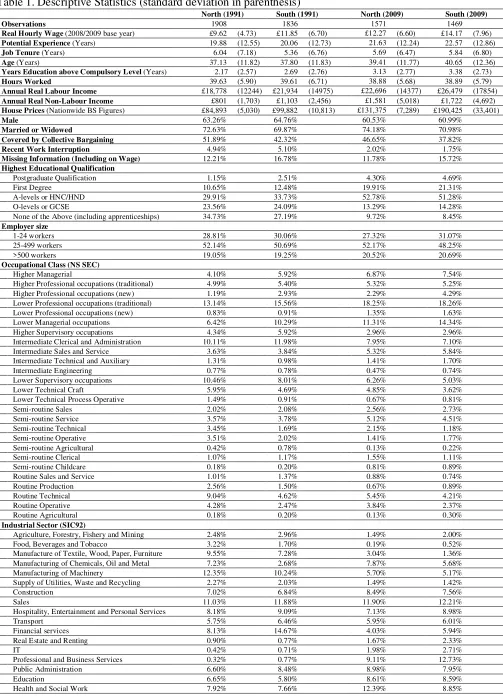
While Table 1 only provides two snapshots of the sample – at both ends of the period –, some important features are immediately observable. The selected sample is very homogenous and mirrors national averages in most demographic characteristics (ONS 2010c). Gender composition is remarkably similar, and there are no statistically significant differences in the means and variances of age, hours worked, potential experience, job tenure and employer size between the regions1 allowing the analysis to concentrate on factors that can be influenced by policy. While non-labour sources are of increasing importance, labour earnings in the sample are still by far the largest source of income with a substantial margin. Most importantly, 1991’s 18.8% gap between average regional wages expressed as a percentage of the Southern wage decreased to 13.4% by 2009, while the initial 27.3% gap in non-labour income dropped to 8.2% by the end of the period. There had been significant inter-regional differences in the years of education above compulsory level in 1991, but due to substantial improvements in Northern educational levels, the gap decreased markedly over the period. A similar pattern emerges with educational qualifications, occupational and industrial structure where the North was in a much less favourable position in 1991, but by 2009 a substantial part of these differences had been eliminated. Despite the extensive convergence in the occupational structure, by 2009 the relative proportion of Southern workers in higher and lower professional, managerial and

1

Table 1. Descriptive Statistics (standard deviation in parenthesis)

North (1991) South (1991) North (2009) South (2009) Observations 1908 1836 1571 1469

Real Hourly Wage (2008/2009 base year) £9.62 (4.73) £11.85 (6.70) £12.27 (6.60) £14.17 (7.96)

Potential Experience (Years) 19.88 (12.55) 20.06 (12.73) 21.63 (12.24) 22.57 (12.86)

Job Tenure (Years) 6.04 (7.18) 5.36 (6.76) 5.69 (6.47) 5.84 (6.80)

Age (Years) 37.13 (11.82) 37.80 (11.83) 39.41 (11.77) 40.65 (12.36)

Years Education above Compulsory Level (Years) 2.17 (2.57) 2.69 (2.76) 3.13 (2.77) 3.38 (2.73)

Hours Worked 39.63 (5.90) 39.61 (6.71) 38.88 (5.68) 38.89 (5.79)

Annual Real Labour Income £18,778 (12244) £21,934 (14975) £22,696 (14377) £26,479 (17854)

Annual Real Non-Labour Income £801 (1,703) £1,103 (2,456) £1,581 (5,018) £1,722 (4,692)

House Prices (Nationwide BS Figures) £84,893 (5,030) £99,882 (10,813) £131,375 (7,289) £190,425 (33,401)

Male 63.26% 64.76% 60.53% 60.99%

Married or Widowed 72.63% 69.87% 74.18% 70.98%

Covered by Collective Bargaining 51.89% 42.32% 46.65% 37.82%

Recent Work Interruption 4.94% 5.10% 2.02% 1.75%

Missing Information (Including on Wage) 12.21% 16.78% 11.78% 15.72%

Highest Educational Qualification

Postgraduate Qualification 1.15% 2.51% 4.30% 4.69%

First Degree 10.65% 12.48% 19.91% 21.31%

A-levels or HNC/HND 29.91% 33.73% 52.78% 51.28%

O-levels or GCSE 23.56% 24.09% 13.29% 14.28%

None of the Above (including apprenticeships) 34.73% 27.19% 9.72% 8.45%

Employer size

1-24 workers 28.81% 30.06% 27.32% 31.07%

25-499 workers 52.14% 50.69% 52.17% 48.25%

>500 workers 19.05% 19.25% 20.52% 20.69%

Occupational Class (NS SEC)

Higher Managerial 4.10% 5.92% 6.87% 7.54%

Higher Professional occupations (traditional) 4.99% 5.40% 5.32% 5.25% Higher Professional occupations (new) 1.19% 2.93% 2.29% 4.29% Lower Professional occupations (traditional) 13.14% 15.56% 18.25% 18.26% Lower Professional occupations (new) 0.83% 0.91% 1.35% 1.63% Lower Managerial occupations 6.42% 10.29% 11.31% 14.34% Higher Supervisory occupations 4.34% 5.92% 2.96% 2.96% Intermediate Clerical and Administration 10.11% 11.98% 7.95% 7.10% Intermediate Sales and Service 3.63% 3.84% 5.32% 5.84% Intermediate Technical and Auxiliary 1.31% 0.98% 1.41% 1.70%

Intermediate Engineering 0.77% 0.78% 0.47% 0.74%

Lower Supervisory occupations 10.46% 8.01% 6.26% 5.03%

Lower Technical Craft 5.95% 4.69% 4.85% 3.62%

Lower Technical Process Operative 1.49% 0.91% 0.67% 0.81%

Semi-routine Sales 2.02% 2.08% 2.56% 2.73%

Semi-routine Service 3.57% 3.78% 5.12% 4.51%

Semi-routine Technical 3.45% 1.69% 2.15% 1.18%

Semi-routine Operative 3.51% 2.02% 1.41% 1.77%

Semi-routine Agricultural 0.42% 0.78% 0.13% 0.22%

Semi-routine Clerical 1.07% 1.17% 1.55% 1.11%

Semi-routine Childcare 0.18% 0.20% 0.81% 0.89%

Routine Sales and Service 1.01% 1.37% 0.88% 0.74%

Routine Production 2.56% 1.50% 0.67% 0.89%

Routine Technical 9.04% 4.62% 5.45% 4.21%

Routine Operative 4.28% 2.47% 3.84% 2.37%

Routine Agricultural 0.18% 0.20% 0.13% 0.30%

Industrial Sector (SIC92)

Agriculture, Forestry, Fishery and Mining 2.48% 2.96% 1.49% 2.00%

Food, Beverages and Tobacco 3.22% 1.70% 0.19% 0.52%

Manufacture of Textile, Wood, Paper, Furniture 9.55% 7.28% 3.04% 1.36% Manufacturing of Chemicals, Oil and Metal 7.23% 2.68% 7.87% 5.68% Manufacturing of Machinery 12.35% 10.24% 5.70% 5.17% Supply of Utilities, Waste and Recycling 2.27% 2.03% 1.49% 1.42%

Construction 7.02% 6.84% 8.49% 7.56%

Sales 11.03% 11.88% 11.90% 12.21%

Hospitality, Entertainment and Personal Services 8.18% 9.09% 7.13% 8.98%

Transport 5.75% 6.46% 5.95% 6.01%

Financial services 8.13% 14.67% 4.03% 5.94%

Real Estate and Renting 0.90% 0.77% 1.67% 2.33%

IT 0.42% 0.71% 1.98% 2.71%

Professional and Business Services 0.32% 0.77% 9.11% 12.73%

Public Administration 6.60% 8.48% 8.98% 7.95%

intermediate occupations is still higher, while Northern workers are still more likely to be employed in less-paid lower technical, semi-routine and routine occupations. In 1991 50.8% of Northern and 64.5% of Southern workers were employed in occupations which required A-level or higher qualifications; by 2009 the proportions changed to 63.5% and 69.7% respectively. With regards to industry structure, while improvements have been significant, marked differences still exist in finance-, professional and business services sectors, while Northern workers are still more likely to work in sectors with relatively lower industry-premium. While the North grew faster in most “good” characteristics, the South too improved its average endowment and was still leading in many categories by 2009.

4.3 The wage gap

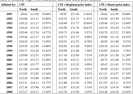
It has been chosen not to adjust wages to regional differences in the cost of living as such indices have only been produced by the Office for National Statistics for two years (2000 and 2004) during the period as a by-product of Europe-wide surveys (Wingfield et al 2005). Using the much more comprehensive Nationwide regional house-price index has also been ruled out, as wages are not meant to compensate for changes in house prices. Table 2’s first column shows the CPI-inflated regional wage-series used in this study, and as an indication its second and third column demonstrates how different the series would have been if the multipliers were applied1. The common feature of all three measures is that they all confirm the existence of an unadjusted pay gap, which seems to be declining over time.

Figures 2 and 3 graph wages from Table 2’s first column and their convergence through the period during which over a quarter of the original wage gap disappeared. Initially the

1

representative Northern worker gets paid 9% below the national average, while its Southern counterpart receives 10% above the mean, but by 2009 the gap shrinks to 6.5% below and 7% above the average, respectively.

Table 2. Inflating wages with local price index and house price inflation

Inflated by: CPI CPI + Regional price index CPI + House price index North South North South North South

1991 £9.62 £11.85 18.80% £9.87 £11.46 13.84% £9.62 £11.85 18.80%

1992 £10.06 £12.11 16.89% £10.32 £11.71 11.81% £10.96 £13.49 18.74%

1993 £10.23 £12.17 15.97% £10.49 £11.77 10.84% £10.48 £12.14 13.69%

1994 £10.24 £12.16 15.81% £10.50 £11.76 10.67% £10.70 £12.10 11.53%

1995 £10.44 £12.24 14.77% £10.71 £11.84 9.57% £10.70 £12.21 12.36%

1996 £10.46 £12.17 14.10% £10.73 £11.77 8.86% £10.00 £11.16 10.45%

1997 £10.26 £11.92 13.95% £10.53 £11.53 8.70% £9.95 £11.00 9.53%

1998 £10.29 £12.09 14.88% £10.56 £11.69 9.69% £10.18 £11.42 10.85%

1999 £10.71 £12.28 12.82% £10.99 £11.88 7.50% £10.05 £10.44 3.78%

2000 £10.90 £12.51 12.85% £11.18 £12.09 7.53% £10.28 £11.58 11.29%

2001 £11.19 £12.73 12.09% £11.48 £12.31 6.73% £9.75 £11.00 11.43%

2002 £11.80 £13.77 14.32% £12.11 £13.32 9.09% £9.42 £11.45 17.73%

2003 £11.88 £13.66 13.05% £12.35 £13.01 5.01% £9.90 £12.63 21.62%

2004 £12.02 £13.85 13.24% £12.50 £13.19 5.22% £11.21 £13.57 17.34%

2005 £12.20 £14.00 12.86% £12.69 £13.33 4.81% £12.20 £14.01 12.89%

2006 £12.31 £14.11 12.77% £12.80 £13.44 4.70% £11.97 £13.11 8.73%

2007 £12.38 £13.96 11.34% £12.87 £13.29 3.14% £13.28 £14.76 9.98%

2008 £12.27 £14.17 13.45% £12.76 £13.49 5.45% £14.48 £16.76 13.64%

Figure 2. Regional gross average real hourly wages of full time employees with reference to the national average (Inflated by CPI, base year: 2008/2009)

Figure 3. Regional gross mean hourly labour wages of full time employees as a percentage of the national average

£9 £10 £11 £12 £13 £14 £15

1991 1993 1995 1997 1999 2001 2003 2005 2007

North South England

90% 95% 100% 105% 110%

1991 1993 1995 1997 1999 2001 2003 2005 2007

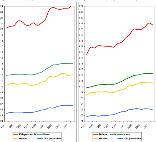
Figures 4 and 5 – by keeping the exact scale of Figure 2 – show that while within region inequalities grew, the between region gaps at selected percentileshave decreased.

Figure 4. Southern gross real average hourly labour wages of full time employees at different points in the wage distribution. (base year: 2008/2009)

Figure 5. Northern gross real average hourly labour wages of full time employees at different points in the wage distribution. (base year: 2008/2009)

£4 £5 £6 £7 £8 £9 £10 £11 £12 £13 £14 £15 £16 £17 £18 £19 £20 £21 £22 £23 £24

1991 1993 1995 1997 1999 2001 2003 2005 2007

90th pe rcentile Mean

Me dian 10th percentile

£4 £5 £6 £7 £8 £9 £10 £11 £12 £13 £14 £15 £16 £17 £18 £19 £20 £21 £22 £23 £24

1991 1993 1995 1997 1999 2001 2003 2005 2007

90th pe rcentile Mean

Me dian 10th percentile

4.4 Insights from the year-by-year OLS results

All coefficients in the year-by-year per-region OLS estimates1 have the expected sign and magnitude. All groups of categorical variables – educational qualifications, employer sizes, occupations and sectors – confirm the expected relation between the group-variables. The specification explains 56% of the variance on average after adjusting for the lost degrees of freedom, with no over-time trend in R2. A very high proportion of coefficients – including the twenty-six occupational and seventeen sectoral dummies – are significant at the 1% level throughout the period. T-tests on the Inverse Mills’ Ratio indicates selection bias in most annual regressions of both regions up to 2002, from which point – may be explained by the increasing female participation levels – it never turns significant again. Although the test statistic decreased over the period, all hypotheses that the coefficient vectors between North and South are not significantly different could be rejected in all years at p0.0001.

While all other coefficients show a definitive trend of convergence, the starkest cross-regional differences, both in absolute terms and in their trend, are found between returns to potential experience, occupations and industry structure, which makes them potential candidates to account for the unexplainable part of the observed pay gap. Northern coefficients on occupational classes increase markedly throughout the period and by 2009 wage premia are higher in almost every occupation in the North. On the other hand, from 2002 onwards Southern returns to experience rise gradually soon becoming over a half larger than the corresponding Northern coefficients. Regions seem to offer slightly higher wages in their traditionally regional industries – e.g. manufacture in the North, finance in the South, but on average Southern industries appear to pay a higher industry wage premium than their Northern counterparts.

1

Figures 6 and 7 show how coefficients on tertiary and secondary qualifications decline considerably in both regions, but remain somewhat higher in the North during the period (O-level / GCSE qualifications are not graphed, as they only exert significant effects on wages through the 1990s). Returns to large employer is higher in the South, while union coverage premium, although declining in both regions, found to be considerably higher in the North. Coefficients on gender gap were initially higher in the North, but fell below Southern levels by 2005.

Figure 6. Over-time change in Northern coefficients of selected categorical variables.

0 0.1 0.2 0.3 0.4 0.5

1991 1993 1995 1997 1999 2001 2003 2005 2007

Tertiary

Secondary

Gender gap

Large Employer

Union

Figure 7. Over-time change in Southern coefficients of selected categorical variables.

0 0.1 0.2 0.3 0.4 0.5

1991 1993 1995 1997 1999 2001 2003 2005 2007

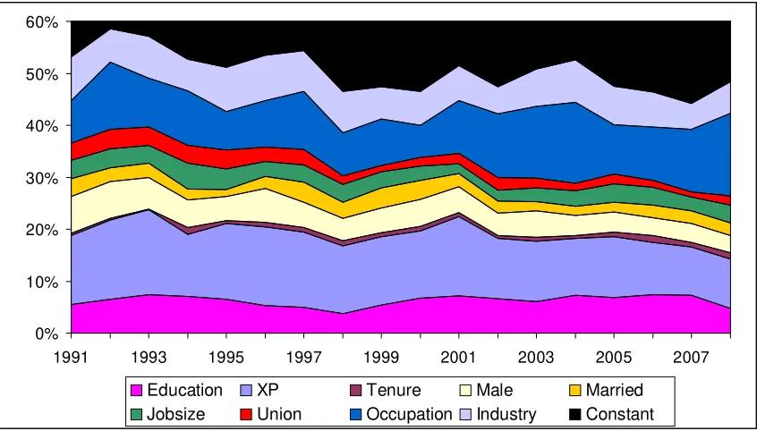
Figures 8 and 9 – by multiplying the coefficient vector with the vector of average characteristics and expressing it as a percentage of the predicted wage – show the relative importance of each groups of variables in predicting the average worker‘s wage year-by-year. The percentages on the graph are therefore not marginal returns. The advantage of

Figure 8. Percentage of Northern average wage predicted by categories of regressors

0% 10% 20% 30% 40% 50% 60%

1991 1993 1995 1997 1999 2001 2003 2005 2007

Education XP Tenure Male Married Jobsize Union Occupation Industry Constant

Figure 9. Percentage of Southern average wage predicted by categories of regressors

0% 10% 20% 30% 40% 50% 60%

1991 1993 1995 1997 1999 2001 2003 2005 2007

such a representation over presenting the change in the coefficients over time is that this approach also takes the changes in the characteristic-means into account. For the average worker (see Table 1) experience is found to be very important in predicting wages, especially in the South. Occupation and industry sector determine around 20% of the mean wage, yet the much higher Northern coefficients on occupational classes do not seem to translate into a stronger effect of occupations in the Northern wage determination implying a lower supply in the high premium occupations and/or a lager supply in the low premium occupations in the North compared to Southern levels. While hardly 6% of the wage can be attributed to education, the relatively stable share of education confirms that the falling coefficients and the increasing participation cancelled each other out in their effect on the wage. Job tenure, gender, marriage, employer size and union premium all decline in importance, but remain somewhat stronger in the North, predicting 10% of the wage by 2009 compared to 7% in the South.

4.5 Oaxaca decomposition results

Figure 10. The relative contribution of the main terms

0% 4% 8% 12% 16% 20%

1991 1993 1995 1997 1999 2001 2003 2005 2007

Interaction term Coefficient gap Endowment gap

The endowment effect, as in Table 31, was initially caused by the fewer workers in high wage-premium occupations and the lower average educational attainment in the North. The results also confirm that much of the educational attainment gap – responsible for over one fifth of 1991’s pay differences – had been eliminated by the end of the 1990s, while the occupational gap – although halved in absolute terms – remained relatively stable in its contribution and in most years accounts for a quarter of the entire pay gap. Industrial structure as a whole is only responsible for a small fraction of pay differentials as a result of

1 _{The decomposition technique used makes it possible to discuss the endowment or coefficient effect of any}

a fine balance between industries with increasing and decreasing individual effects on the gap. The North’s wider union coverage and its initially higher average job tenure only reduce wage differences significantly during the 1990s. Gender, potential experience, marriage and employer size would not exert significant endowment effects on wage gap as these are equally distributed across the regions.

The detailed decomposition results in Tables A.2/1 and A.2/3 show that the occupational gap is mainly caused by the North’s too few workers in managerial and professional positions, and too many workers in routine technical and operative occupations compared to Southern proportions. It can also be seen that the majority of the initial educational gap was not caused by differences in workers with secondary or tertiary certificates, as such differences were nearly insignificant, but by the gradually higher number of workers with no qualifications in the North. The convergence in average educational levels was mainly facilitated by closing this particular gap, and also by slight improvements in the relative proportion of workers with university education. The industry-mix gap has been primarily caused by the North’s too few workers in the high wage-premium financial and IT, and too many workers in the lower premium health sector; however these effects are somewhat counterbalanced by the higher proportion of Northern workers in manufacturing and construction, and fewer workers in hospitality and sales sectors than in the South.

Table 3/1. Oaxaca decomposition results

1991 1992 1993 1994 1995 1996 1997 1998 1999 Log of Wage Gap 0.169 0.167 0.154 0.149 0.146 0.150 0.135 0.139 0.141 Endowment effect 0.071 43% 0.047 29% 0.037 23% 0.027 20% 0.035 26% 0.033 21% 0.024 18% 0.039 28% 0.018 13%

Experience -0.002 -1% -0.004 -2% -0.004 -3% -0.003 -2% -0.001 0% -0.005 -3% -0.005 -3% -0.006 -4% -0.009 -6% Job tenure -0.002 -1% -0.002 -1% -0.003 -2% -0.003 -2% -0.006 -4% -0.005 -3% -0.003 -2% -0.005 -3% -0.008 -6% Educational Attainment 0.021 13% 0.020 12% 0.015 9% 0.014 11% 0.015 11% 0.016 10% 0.009 7% 0.012 9% 0.007 5% Gender Gap 0.000 0% -0.003 -2% -0.002 -1% -0.004 -3% -0.006 -5% -0.002 -1% -0.002 -2% -0.002 -2% -0.001 -1% Collective Bargaining -0.006 -3% -0.007 -4% -0.008 -5% -0.005 -4% -0.011 -8% -0.008 -5% -0.003 -3% -0.003 -2% -0.001 -1% Occupation 0.051 31% 0.041 25% 0.039 25% 0.023 17% 0.034 25% 0.033 21% 0.034 26% 0.044 32% 0.028 20% Industry 0.013 8% 0.009 5% 0.002 1% 0.007 5% 0.010 7% 0.006 4% 0.002 1% 0.001 1% 0.005 4%

Coefficient effect 0.123 74% 0.136 82% 0.14 88% 0.12 88% 0.109 80% 0.124 79% 0.123 91% 0.109 79% 0.131 93%

Experience 0.021 12% -0.060 -37% -0.130 -82% 0.017 12% -0.053 -39% -0.039 -25% -0.006 -4% 0.034 24% 0.002 1% Job tenure 0.004 3% 0.003 2% 0.012 8% -0.005 -3% 0.019 14% 0.007 4% 0.004 3% 0.007 5% 0.020 14% Educational Attainment 0.007 4% -0.016 -10% 0.000 0% 0.002 2% -0.006 -5% -0.039 -25% -0.012 -9% -0.004 -3% 0.006 5% Gender Gap -0.019 -12% -0.037 -23% -0.025 -16% -0.013 -10% 0.005 4% -0.050 -32% 0.015 11% 0.003 2% -0.025 -17% Collective Bargaining -0.027 -16% -0.021 -13% -0.019 -12% -0.031 -23% -0.016 -12% -0.016 -10% -0.039 -29% -0.013 -9% -0.016 -11% Occupation 0.021 13% 0.012 7% 0.049 31% 0.030 22% 0.019 14% 0.012 7% 0.033 25% 0.047 34% 0.019 13% Industry 0.013 8% 0.032 19% 0.013 8% 0.006 4% 0.042 31% 0.028 18% 0.026 19% -0.015 -11% 0.002 1% Intercept 0.115 69% 0.210 127% 0.259 163% 0.122 90% 0.080 58% 0.209 133% 0.113 84% 0.082 59% 0.198 140%

Table 3/2.

2000 2001 2002 2003 2004 2005 2006 2007 2008 Log of Wage Gap 0.127 0.116 0.146 0.126 0.107 0.126 0.107 0.099 0.117 Endowment effect 0.033 26% 0.013 12% 0.026 18% 0.015 12% 0.004 4% 0.008 6% 0.002 2% 0.014 14% 0.033 28%

Experience -0.011 -8% -0.017 -15% -0.016 -11% -0.018 -14% -0.015 -14% -0.011 -9% -0.011 -11% -0.011 -11% -0.003 -2% Job tenure -0.002 -1% -0.001 -1% 0.000 0% -0.003 -3% -0.001 -1% -0.001 -1% 0.000 0% 0.000 0% 0.000 0% Educational Attainment 0.010 8% 0.005 5% 0.008 5% 0.009 7% 0.005 5% 0.004 4% 0.002 2% 0.010 10% 0.002 2% Gender Gap -0.001 -1% -0.001 -1% 0.003 2% 0.000 0% -0.002 -2% -0.001 0% -0.002 -2% -0.005 -5% 0.001 1% Collective Bargaining -0.003 -2% -0.003 -2% 0.000 0% 0.000 0% 0.000 0% -0.001 -1% 0.002 2% -0.002 -2% 0.000 0% Occupation 0.040 31% 0.023 20% 0.033 23% 0.028 22% 0.023 22% 0.016 12% 0.012 11% 0.022 22% 0.025 22% Industry 0.000 0% 0.008 7% -0.001 -1% 0.002 2% -0.005 -5% 0.004 3% 0.004 4% 0.005 5% 0.008 7%

Coefficient effect 0.106 83% 0.113 97% 0.137 94% 0.123 97% 0.107 100% 0.12 96% 0.126 117% 0.091 91% 0.105 89%

the intercept in explaining the regional pay gap. The coefficient effect due to the South’s higher industry premium magnifies pay differences further. Only a third of these effects is counterbalanced by the higher Northern coefficients on union premium, marriage and the

gender gap in most years, as well as coefficients on education and occupational classes towards the end of the period.

The detailed decomposition (Tables A.2/2 and A.2/4) shows that the coefficient effect on education, which works towards reducing the wage gap, develops when Southern returns to

O-level and A-level/HNC/HND qualifications drop substantially around 2002 while it remains relatively stable in the North throughout. The results also confirm that the coefficient effect on industry structure is mainly caused by the higher Southern industry wage-premium in the financial, public administration, transportation and professional services sectors, however the relatively higher Northern premium in manufacturing, education, health and sales sectors somewhat weaken the overall effect. It can be seen that in the 1990s the coefficient effect on occupations further aggravates pay differences, but the tendency is gradually reversing from 2002 onwards, when returns to top occupational classes become markedly higher in the North.

adopting the view that industrial and occupational structure is a possible source of the divide, and accordingly only human capital is accounted for in the analysis, it can be concluded that by the end of the period, the entire pay gap becomes attributable to an unexplainable coefficient effect – or the North-South divide. The analysis, while confirming the existence of the divide, remains largely inconclusive in identifying the sources of such effect, as most of the coefficient differences are caused by the intercept-gap and the very different returns to experience from 1998 onwards. As average experience levels are identical across the regions, this suggests that a large part of the pay gap might be determined by variables not included in the model.

4.6 North-South divide coefficient

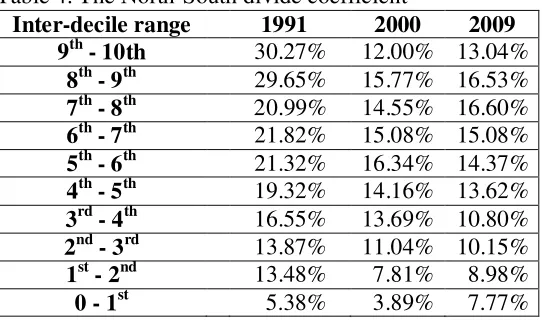
While the paper could stop here, the analysis would be of little use if along the wage distribution the proportion of the forces identified, especially the unexplainable coefficient effects, would be very different. To test how representative previous findings may be along the distribution, a North-South divide coefficient, indicating how much Northern wages would increase in the absence of the North-South divide, is calculated at every inter-decile range in selected years to analyse how different the North-South divide might be upon departure from the means.

Table 4. The North-South divide coefficient

Inter-decile range 1991 2000 2009 9th - 10th 30.27% 12.00% 13.04%

Table 4 shows a strong negative correlation between inter-quantile rank and the size of the unfavourable treatment effect – or the North-South divide; and also confirms a reduction in the unexplainable part of the gap over time in most decile ranges. The relatively even distribution of the coefficient, and the findings suggesting that lower wage groups may experience less of the divide, give some comfort over the applicability of earlier findings across the wage distribution.

4.7 JMP decomposition results

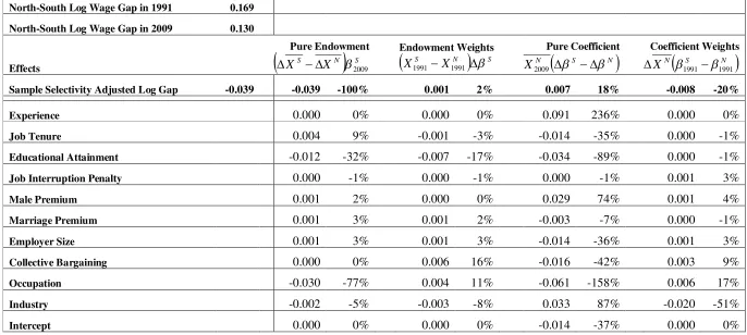
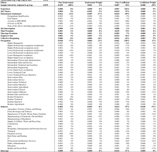
occupational wage-inequality was essential to contain the unexplainable coefficient effect driven by the increase in Southern returns to experience which was so strong, it alone could have offset all effects of the Northern convergence. As components of the coefficient effect operating in either direction are estimated to be four times as strong as the endowment effect, even though their overall effect sums to zero, it has to be acknowledged that the over-time decrease in the wage gap was more of the outcome of a fortunate balance between coefficient effect components, than of improvements in the Northern endowment. The pure endowment effect, or the relative improvements in the North’s measurable characteristics, account for 100% of the decrease in the pay gap over the period. The results (Table 51) confirm earlier findings as these improvements were primarily driven by larger Northern improvements in occupational mix and educational attainment. A slight Northern improvement in the relative industry structure is also traceable.

The detailed decomposition (Table A.3) reveals that the endowment effect on education was due to higher over-time increases in Northern levels of postgraduate, first degree and A-level/HNC/HND qualifications and to the decrease in the proportion of workers with no qualifications. The decrease in the pay gap caused by changes in the relative occupational mix are accountable to larger over-time boosts in the proportion of people working as (in order of importance) lower and higher managers, lower and higher professionals, intermediate administrators and higher supervisors in the North. These developments happened in the traditional professional occupations – such as doctor, solicitor, engineer – as the North’s relative position in modern professional job categories – such as software designer – has worsened over time.

1

Table 5. JMP decomposition results

North-South Log Wage Gap in 1991 0.169 North-South Log Wage Gap in 2009 0.130

Effects

Pure Endowment





X

X  ₂₀₀₉



Endowment Weights





X X₁₉₉₁ ₁₉₉₁ 

Pure Coefficient





N

X₂₀₀₉  

Coefficient Weights





N

X ₁₉₉₁ ₁₉₉₁ 

Sample Selectivity Adjusted Log Gap -0.039 -0.039 -100% 0.001 2% 0.007 18% -0.008 -20%

Experience 0.000 0% 0.000 0% 0.091 236% 0.000 0%

Job Tenure 0.004 9% -0.001 -3% -0.014 -35% 0.000 -1% Educational Attainment -0.012 -32% -0.007 -17% -0.034 -89% 0.000 -1% Job Interruption Penalty 0.000 -1% 0.000 -1% 0.000 -1% 0.001 3%

Male Premium 0.001 2% 0.000 0% 0.029 74% 0.001 4%

Marriage Premium 0.001 3% 0.001 2% -0.003 -7% 0.000 -1% Employer Size 0.001 3% 0.001 3% -0.014 -36% 0.001 3% Collective Bargaining 0.000 0% 0.006 16% -0.016 -42% 0.003 9% Occupation -0.030 -77% 0.004 11% -0.061 -158% 0.006 17% Industry -0.002 -5% -0.003 -8% 0.033 87% -0.020 -51%

opposite direction, and therefore the Northern endowment-convergence could apply its full force in decreasing the pay gap.

Both weight effects are the secondary products of the previously discussed pure effects by acting as weights for their counterparts, therefore discussing them would not add to this analysis especially that their magnitude is very low indeed.

The results, while confirming earlier findings, make them less robust at the same time. The pay gap did decline as an outcome of the North’s remarkable improvements in all measurable areas, but parallel coefficient effects in both directions, four times as strong as pure endowment effects, have also been detected. As the two regions are very homogenous in their potential experience levels, the extremely strong coefficient effect on the variable implies that the wage gap could be largely influenced by over-time changes in unobserved characteristics with which experience levels correlate, suggesting some kind of inter-regional disequilibria, external economies or spill-over effects in the South as an outcome of the 1990s’ unequal human capital distribution.

The conclusion that the coefficient effects of occupations and educational attainment counterbalanced the coefficient effect of returns to experience, and therefore improvements in the Northern endowments could decrease the pay gap, is not the only possible interpretation of the findings. An equally valid argument would be that the increase in the North-South divide was much greater than the improvements in the relative Northern endowments during the period, however the wage gap still dropped, because the within

dispersion, implying that the findings may rather suggest some kind of temporary disequilibrium.

5. Conclusion

The existence of the North-South divide has been confirmed by showing in both static and dynamic analyses that measurable differences in worker and labour market characteristics can only explain a quarter of the pay gap or its change over time. It has been suggested that factors not included in the model could be responsible for as much as half of the unexplained part of the gap. The paper has shown that Southern returns to experience increased so much over the period, that the North’s remarkable catch-up in educational attainment, occupational and industrial structure could only translate into an actual decrease in the overall pay gap, because it coincided with a marked rise among Northern occupational wage premia for top occupations, which increased Northern wages just enough so that wage increases in the South stemming from the higher returns to experience were matched. The quarter decrease in the pay gap over the 1991-2009 period therefore was more of the outcome of an increasing within-region wage inequality, than of the inter-regional convergence in endowment levels, suggesting that the size of the wage gap and its change may be much more dependent on effects that are not directly controllable by policy. Although the increase in the Northern occupational premia for top occupations increased the average Northern wage, did it in an unaccountable fashion, and consequently the observed convergence in the wage levels did not come from sustainable sources. This way, paradoxically, the analysis confirmed a causal relationship between increasing