Exact Solutions of Gardner Equations through tanh coth Method

(1)

http://www.scirp.org/journal/am ISSN Online: 2152-7393 ISSN Print: 2152-7385

Exact Solutions of Gardner Equations through

tanh-coth Method

Lin Lin, Shiyong Zhu, Yinkang Xu, Yubing Shi

Department of Mathematics, Zhejiang Normal University, Jinhua, China

Abstract

In this paper, we apply the tanh-coth method and traveling wave transformation method for solving Gardner equations, including (1 + 1)-Gardner and (2 + 1)- Gardner equations. The tanh-coth method proved to be reliable and effective in han-dling a large number of nonlinear dispersive and disperse equations. Through tanh- coth method, we get analytical expressions of soliton solutions of Gardner equations. The one-soliton solution is characterized by an infinite wing or infinite tail.

Keywords

tanh-coth Method, Gardner Equations, Soliton Solutions

1. Introduction

In the study of nonlinear science, finding the exact solution of nonlinear evolution eq-uations is an important subject. Different methods have their different types of specific applications for nonlinear evolution equations. In recent years many scholars put for-ward and developed several new methods for solving PDEs which based on the original method, such as Hirota’s bilinear method [1], homogeneous balance method [2][3], projective Riccati equation method [4] [5], Jacobi elliptic functions method [6], aux-iliary equation method [7], and separation of variables [8][9][10]. Among them, the tanh-coth method and the sine-cosine method are powerful and widely used in several research works. For single soliton solution, the tanh-coth method is easy to use and has been applied for a wide variety of nonlinear problems.

In the plasma physics, solid physics, fluid mechanics, etc., the Gardner equation is written as

2

0,

t x x xxx

u

+

α

uu

+

β

u u

+

γ

u

=

(1) which is also called the KdV-mKdV equation. The model can be well described the

How to cite this paper: Lin, L., Zhu, S.Y., Xu, Y.K. and Shi, Y.B. (2016) Exact Solu-tions of Gardner EquaSolu-tions through tanh- coth Method. Applied Mathematics, 7, 2374- 2381.

http://dx.doi.org/10.4236/am.2016.718186

Received: October 20, 2016 Accepted: December 19, 2016 Published: December 22, 2016

(2)

wave propagation in a one-dimensional nonlinear lattice with a non harmonic bound particle. Gardner equations have very important application in mathematics, physics, engineering and other fields. Different types of equations can be obtained by changing the value of

α

,

β

, γ .

With

β =

0

,

γ =

1

, the KdV equation is written as

0,

t x xxx

u +αuu +u =

(2)

where the parameter

α

can be scaled to any real number, usually taking α = ±1 or 6

α= ± _{. KdV equation simulates a variety of nonlinear phenomena, including the ion}

acoustic waves and diving waves in the plasma.

With

α

=

0,

γ

=

1

, we get the mKdV equation which is written as 2

0.

t x xxx

u

+

β

u u

+

u

=

(3)

It is completely integrable [11] and can be obtained by Miura transformation of the KdV equation.

The Gardner equations are used to describe many physical models, which are closely related to the study of physics. So it is very important to study it deeply.

With 2

6,

6 ,

1 α

= −

β

= −



γ

=

, the (1 + 1)-Gardner equation turns out to be

2 2

6

0.

t x x xxx

υ

−

υυ

−



υ υ υ

+

=

(4)

Further, the (2 + 1)-dimensional Gardner Equation [12][13][14][15] is written as

2 2 2

3

6 3 3 0

2 ,

t xxx x x y x

x y

ω ω α ω ω βωω γ υ αγω υ

υ ω

+ − + + − =

=

(5)

which reduces to the (1 + 1)-Gardner equation with

ω

_y =0.

For α=0, Equation (5) is transformed into the KP equation as 2 1

6 3 0,

t xxx x x yy

ω ω

₊ ₊

βωω

₊

γ

_∂−

υ

₌

₍₆₎

while it is the modified KP equation with

β =

0

. Therefore, the (2 + 1)-Gardner

equa-tion combines KP equaequa-tion and modified KP equaequa-tion.

With

α

=

2,

γ

= −

1,

β τ

=

, the (2 + 1)-Gardner equation turns out to be

2 1 1

6 6 6 3 0.

t xxx x x x y x x yy

ω ω

₊ ₋

ω ω

₊

ω

_∂−

ω

₊

τωω

_{+ ∂}−

ω

₌

₍₇₎

We had found soliton solutions, travelling wave solutions and plane periodic solu-tions of KdV and mKdV equasolu-tions through tanh-coth method. In order to prove supe-riority of the tanh-coth method, we apply it on Gardner equations which are more complex and have higher dimensions.

This paper is organized as follows. In Section 2, we introduce the tanh-coth method. In Section 3, we first substitute the wave variable

ξ = −

x ct

into the (1 + 1)-Gardner equation, and then integrate once. Based on the tanh-coth method, the soliton and kink solutions of the (1 + 1)-Gardner are given. In Section 4, we would like to search for so-lutions to the dimensionally reduced (2 + 1)-Gardner equation from substituting the wave variable ξ = +x dy−ct. The solutions are obtained by tanh-coth method and the

(3)

2. The tanh-coth Method

A wave variable

ξ = −

x ct

converts any PDE

(

, ,

_t _x

,

_xx

,

_xxx

,

)

0 P u u u u

u



=

(8)

to an ODE

(

, ,

,

)

0. Q u u u u

′ ′′ ′′′



=

(9)

Equation (9) is then integrated as long as all terms contain derivatives where integra-tion constants are considered zeros.

Introducing an independent variable

( )

tanh

,

Y

=

µξ ξ

= −

x ct

(10)

where µ_{is the wave number. The tanh-coth method admits the use of the finite}

ex-pansion

( )

0 1

,

M M

k k

u

µξ

S Y a Y b Y−

= =

∑

+

∑

₍₁₁₎

where M is a positive integer, in most cases, that will be determined by balance

me-thod. And we usually balance the highest order nonlinear terms with the linear terms of highest order by using the scheme given as follows:

,

u→M

, n

u →nM

1,

u

′ →

M

+

( )r _.

u →M+r (12)

Substituting (11) into the reduced ODE results. We then collect all coefficients of each power of _Yk, 0≤ ≤_k _nM_{in the resulting equation where these coefficients have}

to vanish. This will give a system of algebraic equations involving the parameters

, , k k

a b µ and c. Finally, we obtain an analytic solution

u x t

( )

,

in a closed form.

3. The Solutions of (1 + 1)-Gardner Equation

We first substitute the wave variable

ξ = −

x ct

into the (1 + 1)-Gardner equation

(

2 2

)

6 0,

t x xxx

u − u+ u u +u = (13)

that gives

(

2 2

)

6 0.

cu′ u u u′ u′′′

− − + + = (14)

Integrating once to obtain

2 2 3

3 2 0.

cu u u u′′

− − −  + = (15)

We then balance the nonlinear term 2 3

2 u

(4)

highest order derivative u′′_{, that has the exponent} M+2. Using the balance process

leads to

3M =M+2, (16)

that gives

1.

M = (17)

The tanh-coth method allows us to use the substitution

( )

1

0 1 1

, .

u x t =S Y =a +a Y+b Y− (18)

Substituting (18) into (15), collecting the coefficients of each power of Yi, 0≤ ≤i 4,

setting each coefficient to zero, we find

0 2 2 3 2

0 0 1 1 0 0 1 1

:

3

6

2

12 0,

Y

= −

ca

−

a

−

a b

−



a

−



a a b

=

1 2 2 2 2 2

1 0 1 0 1 1 1 1

:

6

2 0,

Y

= −

ca

−

a a

−



a a

−



a b

−

a

µ

=

3 2 2 2

1 1 0

:

3

6 0,

Y

= −

a

−



a a

=

4 2 3 2

1 1

:

2

0. Y

= −



a

+

a

µ

=

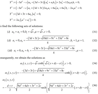
We find the following sets of solutions:

(i) 0 1 0, 1 , , 0,

2 2

c c

a =a = b = − µ= − c< (19)

(ii) 1 0 2 1 2 2

1 1 1 1 1

0, , , , 0,

2 2

2

b = a = − a = µ= c= >



   (20)

(iii) 1 1 2 0 2 2

1 1 1 1

, , , 0.

4

4 2

a =b = − a = − µ= c= >



   (21)

Consequently, we obtain the following solutions:

( )

(

)

1 2

2 1

, tanh , 0,

2 2

u x t = _ x ct− _ c>

  

 (22)

( )

(

)

2 2 2

1 1 1

, coth , 0,

2

2 2

u x t = − + _ x ct− _ c>

  

  (23)

( )

2

(

)

3 2 4 2 2

1 3 2 3

, sech , 0.

2 2 2

c c

u x t = − − − _ − x−ct _ c>

 



   

(24)

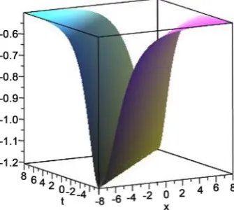
Following immediately. Figure 1 shows a single soliton solution

u x t

3

( )

,

for

1, 1

c= = . In the graph, the X axis is t, the Y axis is

x

, and the Z axis is

u x t

3

( )

,

. It

can be see that the one-soliton solution is characterized by an infinite wing. This shows

that 2

1 2

u→ −

 as

x

and t one of them tends to infinity, that is,

ξ

tends to

(5)

[image:5.595.289.457.73.223.2]

Figure 1. Graph of the one-solution solution u x t3

( )

, for c=1,=1 characterized by an

infi-nite wing.

4. The Solutions of (2 + 1)-Gardner Equation

We first substitute the wave variable ξ = +x dy−ct into the (2 + 1)-Gardner equation

2 1 1

6 6 6 3 0,

t xxx x x x y x x yy

ω ω

₊ ₊

ω ω

₊

ω

_∂−

ω

₊

τωω

_{− ∂}−

ω

₌ ₍₂₅₎

that gives

2 2

6 6 6 3 0

x

cω ω ω ω dω υ τωω d υ

υ ω

− ′+ ′′′+ ′+ ′ + ′− ′=



 _′

= 

Based on

x x

υ

_{υ ξ υ}

ξ

∂ ₌∂ _⋅∂ ₌ _′

∂ ∂ ∂ , we get

2 2

6 6 6 3 0.

cω ω′ ′′′ ω ω′ dωω′ τωω′ d ω′

− + + + + − = (26)

Integrating once to obtain

(

2

)

(

)

2 3

3 3 3 2 0.

c d ω d τ ω ω ω′′

− − + + + + =

(27)

We then balance the nonlinear term 3

2ω , that has the exponent 3M, with the

highest order derivative ω′′, that has the exponent M+2. Using the balance process

leads to

3M =M+2, (28)

that gives

1.

M = (29)

The tanh-coth method allows us to use the substitution

( )

1

0 1 1

, .

x t S Y a a Y b Y

ω

₌ ₌ ₊ ₊ −

₍₃₀₎

Substituting (30) into (27), that gives

(

)(

)

(

)

(

)

(

)

2 1 2 2 3 2 3

1 0 1 1 1 1

2 3

2 1 1 1

1 1 0 1 1 0 1

3 2 2 2

2 3 3 2 0.

d c a Y a b Y a Y a Y b Y

b Y d a Y a b Y a Y a b Y

µ µ µ

µ τ

− −

− − −

− − + + − + +

− + + + + + + + =

Collecting the coefficients of each power of Yi, 0≤ ≤i 4 and then setting each

(6)

(

)

(

)

(

)

0 2 2 3

0 0 1 1 0 0 1 1

: 3 3 3 2 12 0,

Y = − d −c a + d+ τ a +a b + a + a a b =

(

)

(

)

1 2 2 2 2

1 0 1 0 1 1 1 1

: 3 3 3 2 6 6 2 0,

Y = − d −c a + d+ τ a a + a a + a b − aµ =

(

)

3 2

0 1

: 3 3 6 0,

Y = d+

τ

+ a a =

(

)

4 2 2

1 1

: 2 0.

Y = a µ +a =

We find the following sets of solutions:

(i)

a

0

= =

a

1

0,

b

1

=

c

,

µ

=

c c

,

>

0,

(31)

(ii)

(

)

2 2

1 0 1

3 3 18 9 33 8

0, , 1, 1,

4

d d d c

a = a = − +

τ

+

τ

+

τ

+ + b =

µ

=

(32)

(iii)

(

)

2 2

1 0 1

3 3 18 9 33 8

0, , 1.

4

d d d c

a = a = =b − +

τ

+

τ

+

τ

+ +

µ

= (33)

Consequently, we obtain the solutions as

(

)

(

)

1 x y t, , ccoth c x dy ct ,c 0,

ω = _ + − _ >

₍₃₄₎

(

)

(

)

2 2

(

)

2

3 3 18 9 33 8

, , coth ,

4

d d d c

x y t

τ

x dy ct

ω

= −− + + + + + _ + − _ ₍₃₅₎

(

)

(

)

3

2 2 2 2

, ,

9 6 3 2 9 6 3 2

sech ,

2 2 2

x y t

d d d c d d c

x dy ct

ω

τ



τ



+ + + + + + +

= − +  + − 

 

 

(36)

where ω1 and ω2 are kink solutions. And the kink solution’s graph is changing along

with b1 taking different values.

Following immediately. Figure 2 below shows the one-soliton solution

ω

3

(

x y t

, ,

)

for

c

=

1,

d

=

1,

τ

=

1,

t

=

1

. From the graph we can see, the one-soliton solution is cha-

racterized by infinite tail. This shows that

2

d τ

ω→ − + _as

x

and t one of them

[image:6.595.211.556.71.402.2]

tends to infinity, that is,

ξ

tends to infinity.

(7)

5. Conclusion

In this paper, we obtain the soliton and kink solutions of the (1 + 1)-Gardner equation and (2 + 1)-Gardner equation through the tanh-coth method. The biggest advantage is that by traveling wave transformation, the problem of solving nonlinear partial rential equations is transformed into the problem of solving nonlinear ordinary diffe-rential equations or nonlinear algebraic equations. The tanh-coth method is convenient to use, and can be further extended to solve other nonlinear partial differential equa-tions.

Acknowledgements

The authors would like to express their sincere thanks to the referees for their enthu-siastic guidance and help. This work is supported by the National Natural Science Foundation of China (No.11371326)

References

[1] Hirota, R. (2004) The Direct Method in Soliton Theory. Vol. 155, Cambridge University Press, Cambridge. https://doi.org/10.1017/CBO9780511543043

[2] Wang, M. (1995) Solitary Wave Solutions for Variant Boussinesq Equations. Physics Letters A, 199, 169-172. https://doi.org/10.1016/0375-9601(95)00092-H

[3] Fan, E.G. (2004) Integrable Systems and Computer Algebra. Science Press, Beijing.

[4] Ying, J.P. and Lou, S.Y. (2003) Multilinear Variable Separation Approach in (3 + 1)-Dimen- sions: The Burgers Equation. Chinese Physics Letters, 20, 1448.

https://doi.org/10.1088/0256-307X/20/9/311

[5] Fang, J.P. and Zheng, C.L. (2005) New Exact Excitations and Soliton Fission and Fusion for the (2 + 1)-Dimensional Broer-Kaup-Kupershmidt System. Chinese Physics, 14, 669. https://doi.org/10.1088/1009-1963/14/4/006

[6] Liu, S., Fu, Z., Liu, S. and Zhao, Q. (2001) Jacobi Elliptic Function Expansion Method and Periodic Wave Solutions of Nonlinear Wave Equations. Physics Letters A, 289, 69-74. https://doi.org/10.1016/S0375-9601(01)00580-1

[7] Taogetusang, S. (2006) New Type of Exact Solitary Wave Solutions for Dispersive Long- Wave Equation and Benjamin Equation.

[8] Tang, X.Y. and Liang, Z.F. (2006) Variable Separation Solutions for the (3 + 1)-Dimen- sional Jimbo-Miwa Equation. Physics Letters A, 351, 398-402.

https://doi.org/10.1016/j.physleta.2005.11.035

[9] Zhang, S.L., Lou, S.Y. and Qu, C.Z. (2006) The Derivative-Dependent Functional Variable Separation for the Evolution Equations. Chinese Physics, 15, 2765-2776.

https://doi.org/10.1088/1009-1963/15/12/001

[10] Ma, H.C., Ge, D.J. and Yu, Y.D. (2008) New Periodic Wave Solutions, Localized Excitations and Their Interaction for (2 + 1)-Dimensional Burgers Equation. Chinese Physics B, 17, 4344. https://doi.org/10.1088/1674-1056/17/12/002

[11] Malfliet, W. (1992) Solitary Wave Solutions of Nonlinear Wave Equations. American Jour-nal of Physics, 60, 650-654. https://doi.org/10.1119/1.17120

(8)

https://doi.org/10.4236/jamp.2015.36083

[13] Wazwaz, A.M. (2007) New Solitons and Kink Solutions for the Gardner Equation. Com-munications in Nonlinear Science and Numerical Simulation, 12, 1395-1404.

https://doi.org/10.1016/j.cnsns.2005.11.007

[14] Konno, K. and Ichikawa, Y.H. (1974) A Modified Korteweg de Vries Equation for Ion Acoustic Waves. Journal of the Physical Society of Japan, 37, 1631-1636.

https://doi.org/10.1143/JPSJ.37.1631

[15] Chen, Y. and Yan, Z. (2005) New Exact Solutions of (2 + 1)-Dimensional Gardner Equation via the New Sine-Gordon Equation Expansion Method. Chaos, Solitons & Fractals, 26, 399- 406. https://doi.org/10.1016/j.chaos.2005.01.004

Submit or recommend next manuscript to SCIRP and we will provide best service for you:

Accepting pre-submission inquiries through Email, Facebook, LinkedIn, Twitter, etc. A wide selection of journals (inclusive of 9 subjects, more than 200 journals)

Providing 24-hour high-quality service User-friendly online submission system Fair and swift peer-review system

Efficient typesetting and proofreading procedure

Display of the result of downloads and visits, as well as the number of cited articles Maximum dissemination of your research work

Submit your manuscript at: http://papersubmission.scirp.org/