Munich Personal RePEc Archive
Neither easy nor impossible: Local
development economics and policy
Seravalli, Gilberto
University of Parma (Italy)
10 August 2011
Online at
https://mpra.ub.uni-muenchen.de/32743/
NEITHER EASY NOR IMPOSSIBLE:
LOCAL DEVELOPMENT ECONOMICS AND POLICY
By
Gilberto Seravalli
Translation from the Italian to English by
Clarissa Botsford
Introduction ... 3
Chapter One - Territorial disparities ... 9
The basic model: the effects of distance and location... 14
The basic model: dynamics... 20
Some extensions ... 27
Two examples ... 30
The conclusions reached by NEG ... 35
Bibliography for Chapter 1 ... 36
Chapter 1 Appendix 1 - Regional disparities in Europe ... 38
European integration and cohesion: theory ... 39
European integration and cohesion: policies and trends ... 45
Bibliography for Chapter 1 Appendix 1 ... 48
Chapter 1 Appendix 2 - Getting growth going: industrial districts ... 52
Bibliography for Chapter 1 Appendix 2 ... 60
Chapter Two - Underdevelopment Traps and Social Traps ... 63
Underdevelopment traps, the mechanism ... 63
Underdevelopment traps in economic literature ... 65
Social traps ... 67
Combined traps: a model inspired by classical economics ... 71
The basic model: constant techniques ... 72
Second version: endogenous costs ... 76
Development policies ... 79
A multi-agent simulation ... 82
Bibliography for Chapter 2 ... 84
Chapter Three - Collective Goods ... 86
The limits of collective action ... 88
Bottom-up collective action: building cooperative norms ... 90
A promise is a promise ... 93
Conditions and consequent constraints ... 93
Information and coordination costs ... 94
Synchronisation costs ... 95
Selection costs ... 96
Bottom-up collective action: club goods ... 97
Institutional authority... 100
The limits of public intervention ... 101
Choice of managers ... 102
Fiduciary duties ... 105
Employment constraints ... 106
Equity constraints... 106
The measurement of results and the problem of planning and control ... 109
Conclusions ... 114
Bibliography for chapter 3 ... 114
Chapter 3 Appendix 1 - Misiones: a case study of collective action failure ... 116
A little history ... 120
Poverty ... 124
Yerba mate ... 126
The land ... 127
The production process ... 128
Large distribution... 131
Demand ... 132
Supply: the end of the line ... 132
Supply: the beginning of the line ... 132
A vicious circle ... 134
State interventions ... 135
The debate... 137
Bibliography for chapter 3 appendix 1 ... 140
Chapter Four - Institutional Action ... 141
Development policies and decentralisation ... 142
The basic model ... 144
Lagging regions ... 150
Chapter 4 Appendix 1 - The Historical Role of Local Institutions in Italy. ... 158
Chapter 4 Appendix 2 - A Critique of the Cultural Approach. ... 162
Bibliography for chapter 4 ... 165
Chapter Five - Institutional Frameworks ... 168
Decentralisation and resources for local policies ... 170
Simple rules ... 174
Simple rules with difficult final results ... 176
Costs and benefits of learning ... 181
Limited learning costs ... 187
High learning costs ... 187
Designing institutional arrangements ... 189
Bibliography for chapter 5 ... 193
Introduction
This assai leads the reader on an analytical path to development, with institutions as
its central focus. While its main emphasis is on the problematic nature of
development in lagging or backward regions, contributions from the literature on
developing countries have also been taken into account, and European countries, Italy
and the South of Italy (the Mezzogiorno) also feature in the debate. There is no doubt
that lagging regions in advanced countries are very different from backward regions
in poor countries. I think that there are two basic assumptions that hold for both. First,
the most important constraints on development are internal; second, in order to
combat underdevelopment strong actions that break with tradition are needed. These
two assumptions are often ignored by development literature. These studies may be
well written, fun to read and able to communicate faithfully their authors views on
social and economic life, but their perspective is necessarily different from that of
people who are actively involved in social and economic development efforts or
tackling underdevelopment. The assai offers some interpretative starting points. The
path distances itself from five concepts that are widely held but superficial.
The first is that economic development in a backward or lagging area depends on
growth in advanced areas, given that capital will flow where there is an abundant
supply of labour and because technical progress is easier for latecomers than for
innovators. The common view is that there is spontaneous economic convergence
simply because capital has low returns in advanced areas and high returns in
backward areas. In advanced areas, moreover, already on the threshold of improved
technology, technical progress is more of a struggle, whereas in backward areas all
that is needed is to imitate others. Since this idea has no real empirical basis, those
who hold this view claim that the differences between regions persist because markets
work badly, segmented as they are by rules and behaviour that allow unjustified
returns. Without these artificial distortions, they argue, resources would be
spontaneously used where they were most productive. In this view, the most relevant
development policy (and for many, the only possible policy) is to reduce curbs to
maximum competition in all sectors and in all walks of life.
There are many reasons for thinking that this is irrelevant. Many crucial resources
anything, the opposite. Opening up markets that work well would therefore seem to
be a result of development rather than a way to achieve it. In order to achieve
development what is needed is more intentional public intervention: more State, not
less.
The path undertaken to reach this conclusion is arduous, however. Not many people
today share the view that the State can play a relevant role. The path requires a critical
reappraisal of four other common views. The second widespread view that we need to
demolish, then, is the idea that -. even if we accept that economic development in a
backward area is impeded by the fact that resources are attracted to advanced areas -
there will always be immobile resources that can spontaneously trigger development
and sustain it. This view is supported by the limits on mobility of resources. Taking
into account that important resources such as the environmental, historical, cultural
heritage of a region are substantially immobile, those who hold this view believe that
these resources cannot be lost as a result of the capacity for attraction of an advanced
area. They believe that these immobile resources sooner or later will stimulate those
who know how to exploit them effectively and profitably. The reason why this view is
unhelpful is that existing immobile resources can and often do remain inaccessible.
Potentially profitable resources never actually become useful for development
because the conditions for exploiting them have not been achieved, or nobody has
ever thought of using them. A case study illustrating how this can happen is presented
in the Appendix of Chapter Three.
Proceeding along our path, a third commonly held view must be set aside. Even if
they accept that the process of valorising immobile resources is not always so easy,
economists often say that this is not a problem if in the backward area the cost of
labour is very low. The objection is that the difficulty of valorising immobile
resources is made up for by a particularly advantageous condition of low labour costs.
If there were no institutions keeping wages artificially high, unemployment or
under-employment would be solved by salaries so low that the labour cost per production
unit would be advantageous even in situations of low productivity. This, people claim,
would help overcome other curbs on development. This approach is on the surface
quite correct, but it neglects to take into account one feature. Low labour costs could
well get an area out of underdevelopment, but there are no guarantees that if will keep
It is thus necessary to deal with the fourth widely help view. Admitting, at this
point, that underdevelopment in a backward area cannot be overcome spontaneously,
even where there are low labour costs, and accepting that development needs an
action that breaks with tradition, then, it is claimed, bottom-up collective action on the
part of civil society can provide precisely this break. Those who hold this view
believe that in order to trigger and sustain a development process collective goods
such as, for example, material and immaterial infrastructures, insurance, training, and
promotional services, are essential. They do not feel, however, that corresponding
public action is needed. They are convinced that, collectively, civil society can
achieve the goods and services needed. This idea ignores the serious difficulties that
bottom-up collective action meets with if it is not supported by public action, as
Chapter Three illustrates.
This brings us to the fifth and final point of view that we need to deal with.
Admitting that bottom-up collective action is unsuccessful, a break with tradition can
be guaranteed simply by decentralising institutions, providing local authorities with
the sufficient skills and resources to take care of their own needs. We argue that
decentralizing on its own is not a solution. Development policies require State
intervention to be organized in a complex institutional framework, as Chapter Five
shows.
The assai‟s five chapters are each devoted to one of these themes, while the sixth provides a conclusion and completes the arguments set out in the Introduction. The
themes are: territorial imbalances, underdevelopment traps and social traps, collective
goods and services, institutional action and institutional frameworks. Every theme is
supported with an analytical argument and development policy proposals that emerge
as a result.
In Chapter One, territorial imbalances are explained. Space is an obstacle, but not
an absolute barrier to the free movement of goods, people and firms. All that is
needed, then, is for a process of economic growth to be triggered, after which it
becomes cumulative and attracts activities and resources from other places. Backward
areas not only do not receive new resources, they lose the few resources they have,
remaining underdeveloped even when at a national level there is growth. New
based on partial economic equilibrium did not do enough to explain these cumulative
processes. Individual agglomeration factors were identified without placing them in
context. On the other hand, the findings of NEG imply that general equilibrium is
inefficient when territorial development gaps are not temporary. If it is not efficient,
how are these gaps to be closed? NEG makes one suggestion, based on its own
models. In backward areas there are usually unexploited immobile resources that
could be put to use in order to trigger development. The literature on industrial
districts gives an interesting indication of the nature of these immobile resources and
what mechanisms translate into factors of development. These include professional
and organisational resources, which in other areas are mobile but which in these
districts take on a special cohesion (or functional coherence), to the extent that they
adopt the same features as immobile resources in the sense that if they were used
elsewhere they would not be as productive.
The first part of Chapter Two considers underdevelopment traps. While reallocating
resources from less productive to more productive uses may trigger a process of
growth, the related costs may be so high that growth is unlikely to take place – either spontaneously or gradually – because a block of a significant size would have to be reallocated at the same time. This argument can be countered by the observation that
low labour costs compensate for these costs. If labour costs are low owing to
unemployment, then total reallocation costs are not very high. Reallocation takes
place gradually, without any thresholds and without any underdevelopment traps. But
this means ignoring the problem of social traps, which are examined in the second
half of Chapter Two. Low labour costs may facilitate the exit of resources from less
productive uses but in the end they will stop them from staying in more productive
uses. And yet, low labour costs imply an absence of barriers to entry for more
productive uses, with the result of rapidly exhausting existing potential by impeding
sufficient accumulation. Escaping from combined underdevelopment and social traps
requires actions that markets are unable to support, even taking into account
opportunities for exploiting existing resources and the low cost of labour. What is
needed is to allow labour costs to rise and thus overcome reallocation costs that have
thus become so significant. What is needed are collective goods, which provide an
injection of benefits such that people and organisations are able to take on the
with the risks and difficulties inherent in transformation so that they can distance
themselves from the static but guaranteed structure of backward societies.
Chapter Three is devoted to the theme of collective goods in underdeveloped
contexts. The first part of the chapter examines the possibility that collective goods
are realised by those who need them, and concludes that this only happens under very
strict conditions, which do not apply to backward areas. The main obstacle is the lack
of information, which is a problem even in advanced economies but it is exacerbated
in situations of underdevelopment. The inevitable result is that collective goods need
to be public goods. Institutions that contribute to development by establishing public
goods, not just by enforcing regulations, thus become central to any analysis of how
underdeveloped areas can trigger the growth process. The chapter argues, however,
that these active institutions cannot be considered a solution, even assuming that they
are virtuous and not predatory. If imperfect information and uncertainty call for
institutional intervention, this intervention will in its turn be a victim. In particular, as
the chapter goes on to show, a central State that adopts vertical and sectorial
interventions is especially inefficient.
In Chapter Four the question of decentralisation is analysed, taking as given that
institutions should be more accountable and closer to the citizenry. Applying the
criterion of subsidiarity, it would be easy to believe that the more resources local
institutions are endowed with, the more effective their actions will be for
development, and the better they will be able to sustain and support the role of civil
society. The widely held belief, in this case, is that by pursuing pluralism and
democracy, development will automatically follow. Those who reject the orthodox
economic view that all that is needed for development to take off is a functioning
market often adopt this paradigm. And yet, as Chapter Four demonstrates, in
conditions of uncertainty, the proximity of local institutions to specific interest groups
generates a problem of consensus and increases the complexity of the institutional
action needed. The result is that institutional action, which is anyway conditioned by
the history, skills and experience of its managers, is undetermined and leaves plenty of space for „institutional entrepreneurship‟, which may or may not be successful.
Chapter Five is based on the idea that institutional entrepreneurship can be
encouraged, in a decentralised context, by a multi-level organisation of the State,
personnel and functions that allow local systems to communicate constantly with the
outside world in order to obtain additional resources and grasp new opportunities.
This requires a complex institutional framework, which on one hand is essential for
gaining resources, but on the other generates learning costs that can easily lead to
actions that are ineffective for development. The institutional framework also
provides a solution, however, if certain conditions are fulfilled. These are: carefully
designed rules, a realistic expectation of results, continuous monitoring and
evaluation. This path is very different from pure and simple decentralisation because
it implies a strong input from the centre, and an emphasis on inter-institutional
coordination rather than bottom-up policies per se.
The assai has various readers in mind. It is aimed at students in further education,
and in particular in graduate programmes. But it is also intended for people actively
Chapter One - Territorial disparities
1Traditional growth economics is based on the principle that differences in per
capita income among countries or among regions of the same country depend mainly
on differences in capital endowment per worker. And yet, in a context of open
economies, with mobile production factors, and in particular mobile capital,
neoclassical growth economics has not been able to explain why these per capita
differences live on, or even degenerate. In the neoclassical approach, income gaps
lead to even gaps in the rate of returns on capital, dictating that large flows of capital
should be sent from more advanced areas to more backward areas in order rapidly to
reduce these disparities. With a production function in which labour and capital are
substitutes, even when substitution elasticity is equal to one2, and returns of scale are
constant, the rate of return on capital of a backward area whose per capita income is a
tenth3 of an advanced area would be 215 times greater4. The rate of return on capital
income would be double in an area whose per capita income is only slightly lower
(80%) than the more advanced area.
Evidently, the principles of neoclassical economics, especially constant returns of
scale and decreasing returns of capital, do not reflect real life. In more recent growth
economics, these two factors have been removed and new production factors have
been introduced, in particular human capital. Thus up to 60% of per capita income
differences can now be explained, whereas the traditional model only justified 25%
(Lasagni, 2006; Psacharopoulos-Patrinos, 2002; Caselli, 2004). Regional economics5
is better suited to our purposes because it focuses on the relationships between open
economies at a territorial level. Before Krugman‟s contribution (1991), regional economics did not have a convincing answer to the question of why production tends
to agglomerate in certain areas, leaving other areas behind and preserving disparities
1
Sections 1,2 and part of 5 were written with Mario Menegatti
2
With elasticity less than one, which is more realistic to assume, the results would be even more surprising.
3
The poorest country in a sample of 78 nations had an average in the period between 1990-2000 of 3% of the per capita income of the richest country with purchasing power parity (Lasagni 2006). From 1995-2000 in Italy, Calabria – the poorest region – had an average of 44% of the per capita income of the richest region, Emilia-Romagna. Bank of Italy data.
4
With a share of capital income of 30% and thus a labour income of 70%.
5
in regional development.6 Partial equilibrium analyses identified a number of
agglomeration factors. There were not only the natural advantages of certain regions
to take into account - greater natural resources, historical concentrations of
populations, favourable geographic positions – but many other factors. These included Marshall‟s externalities,7 Hirschman‟s linkages in economic activities,8
cumulative processes of increasing returns of scale, a series of divergent forces
leading to dispersion, such as the various categories of congestion costs (Christaller,
1933; Henderson, 1974), as well as transport costs. On the other hand, general
equilibrium analyses were anchored in mainstream international trade theory, which
attempted to explain sectorial specialisation rather than development.9 General
equilibrium models yielded indeterminate results for transport costs, non-competitive
markets and increasing returns. In these models, restrictive (or unrealistic) hypotheses
were often adopted: returns of scale were considered constant, space was either
considered insurmountable (for productive factors) or, by contrast, irrelevant (for
products).10 Thus, while regions in partial equilibrium analyses were allowed to be
historically, geographically, socially and economically specific - and thus have a
variegated profile - these specificities in general equilibrium analyses were reduced
essentially to the different relative endowments of production factors. In the standard
model, production factors were assumed to be immobile. This made for a rather
peculiar vision of history. Before there was any external trade, autarchic regions were
explained by their history; their specific history was both the cause and the
6 The statement that “productive activities tend to concentrate in certain areas... thus preserving
differences in regional development” should be discussed. In highly industrialised countries, and in the
United States in particular, the process of economic development took place at the same time as a marked reduction in regional differences. It is important then to consider what conditions contribute to regional convergence and then see how permanent the disparities are. The Appendix contains a brief contribution with specific reference to Europe.
7
Marshall, 1920
8
Hirschman, 1963
9
The importance assigned to concepts of open economies and international specialisation in international trade theory justified these applications for the simple reason that regions within a country are, by administrative definition and for objective de facto reasons, open economies. The title of one of the most important contributions to international trade theory (Ohlin, 1933: Interregional and International Trade) indicated that the application of his theoretical framework was possible for regions as well as internationally.
10
On a similar basis, general equilibrium analysis showed that international and inter-regional trade
could be considered a “perfect substitute” for the mobility of productive factors. The consequence was
justification for their economic and social differences. Once there was external trade,
however, history was no longer relevant. A new route was taking shape where deeply
lying forces made those differences disappear.
New Economic Geography (NEG), from Krugman‟s contribution in 1991 onwards, reconciled general equilibrium theory with the well-known results of partial
analyses.11 In NEG models, space no longer had the simplified dichotic relevance
whereby in some markets mobility was perfect and in others it did not exist. NEG
assumed, more realistically, that spatial distance always costs something to overcome.
The result was a richer and less simplistic definition of regional differences that
envisaged imperfect mobility both of products and factors. Agglomeration processes
of different production factors and products, and therefore externalities, increasing
returns of scale and finally non-competitive markets, could thus take place. At the
same time, solutions depended on the equilibrium of economic forces both in terms of
concentration and in terms of dispersion.12
To sum up, mainstream international trade theory, from Riccardo to Ohlin, tended
to interpret exchanges between economies as the result of their production
specialisations. These specialisations were explained either on the basis of different
technologies, or on the basis of different endowments of factors - such as, for
example, natural resources and populations – or again, on the basis of relative advantages in producing different goods. Goods markets were generally characterised
by full mobility, while production factor (or resource) markets had zero mobility. It
11It is easy to see why NEG has at times been considered “old wine in new bottles” (Smutzler, 1999,
p.358); but it is also clear why it is important.
12 “Reduced to its essence, the new economic geography is a theory of the emergen
was still not clear what role transport costs and company location played in markets,
although these factors were recognised as being important.13 Traditionally,
international trade theory focused less on agglomerations of production and the
effects of reducing transport costs, and more on the international division of labour in
terms of specialisation in order to stress its greater economic efficiency compared to
autarchic structures.
Starting with Krugman‟s contribution in the early 1990s, NEG attempted to find reasons for geographic location and for the tendency of industrial production to concentrate in some areas rather than others. NEG‟s main departure from the literature regarding international (and inter-regional) trade was to attribute importance
to the distance between production location and markets in which output is sold and
inputs are bought. Firstly, NEG took account of the fact that selling goods in a
different location from where they are produced incurs costs related to packaging,
preserving, and transporting goods, as well as to the documentation and
administration of the contracts required when the buyer has no direct control over the
quality, quantity or nature of the product, and the seller does not receive the revenues directly. These “transport costs” mean that from a company‟s point of view, different locations represent different markets, in the sense that the company provides the same
goods at differing costs. Secondly, NEG recognised the fact that there are scale
economies and that the structure of markets is not perfectly competitive, meaning that
the level of demand for goods produced by one company is influenced by the location
of other producers. Thirdly, these assumptions, together with the existence of
input-output links between companies, imply that the cost of buying intermediate goods
used in production depends on the location of suppliers.
These intuitions allowed NEG to identify the forces at work behind the
agglomeration of production in certain areas, as well as to recognise the divergent
forces that contribute to dispersion. When forces that induce firms to concentrate in
certain areas prevail, a self-reinforcing mechanism - whereby links between
production and demand for goods, and between production of final goods and
production of intermediate goods, are often forged - leads to further agglomeration.
13“International trade cannot be understood except in r
elation to and as part of the general location
NEG was able to recognise when this mechanism had been set in motion and at the
same time to identify the factors that initiated or hindered the process.
The agglomeration mechanism described by NEG played a significant role in the
way local development was analysed for two reasons. First, NEG evidenced that
mobile resources tended to migrate towards more developed areas; in under
developed regions, NEG concluded, it was preferable to concentrate interventions on
immobile resources. Second, it stressed that, once the mechanism was set in motion,
the process could become self-reinforcing by attracting new companies. The
contribution of NEG to the debate on developing backward regions was by no means
definitive, but it did forge new analytical paths. On the one hand, there was the matter
of determining how to set the mechanism in motion; on the other, the question of
identifying what conditions favour or hinder the mechanism once it has been
triggered. The innovative factor in the debate, in contrast to mainstream ideas of
economic development, was the idea that economic development in a region is a
process that is difficult to set in motion, but that once it has been triggered, it can
become self-reinforcing and even accelerate, unless obstacles come in its way, or
attrition slowly blocks the mechanism. This idea contrasted with prevalent thinking in
mainstream economic development approaches, which considered the country as a
whole. The accepted view was that historical circumstances, more than anything else,
determined whether local development could be set in motion very easily or with
great difficulty. According to this view, once it had started, development proceeded
in a regular fashion, without any particular acceleration or any relevant slow downs.
The justification for this view was that a local system was more open and
inter-dependent. Every local system was susceptible to being hindered or encouraged by
other local systems. It could be hindered if it were weak,14 because it would lose
resources to others; it could be encouraged as long as it were strong, because the
resources of other systems would naturally flow towards it.15 When a „national‟ economic system was considered as a whole, the positive or negative effects of
inter-dependence in its regions were not taken into account.
14
A weakness at the beginning, as we shall see, can also become a strength if there exists a potential to exploit and if it is effectively exploited. A historical strenght can also become a weakness if, for example, congestion costs become prevalent.
15
inter-Sections one and two present a simplified version of the issues examined by NEG,
with reference respectively to the structure of models and the consequences of firms‟ location choices. Section three examines some important extensions. Section four
gives two concrete examples, while section five summarises the conclusions.
The basic model: the effects of distance and location
The objectives of NEG‟s analysis of development can be summarised as follows: to identify the effects of distance between production and its buyers and
suppliers and examine the consequences of location choices
to identify the forces that lead to agglomeration of companies in certain areas rather than others, as well as the forces that work against this concentration
to indicate the factors behind these forces.
In order to examine the effects of distance between production and its markets, it is
important to identify the elements that make location economically significant. With
this aim in mind, let us simplify the matter and consider two economies (A and B) that produce two goods: one agricultural or „traditional‟ product (such as wheat) x, and one industrial or „modern‟ product (such as cars), y. We will begin by examining a case in which distance is irrelevant. It can be demonstrated that the distance between
production and markets is not relevant if the following assumptions hold.
First assumption. Both goods, wheat and cars, are produced with different
technologies but with constant returns of scale. Put simply, a production function can
be imagined in which the only input is labour. When there is only one input, the
hypothesis of constant returns of scale means that the relationship between output and
input is constant. The production functions of wheat (x) and cars (y) in cases like this
are:
x
l
x with 0 [1]
y
l
y with 0 [2]
where lx e ly represent the labour used to produce each good.
Second assumption. Each of the two goods is produced by each of the two
economies and they make their choices on the basis of a given market price. In this
Third assumption. The optimal choice for each consumer is made on the basis
of personal choices. Put simply, these can be summarised as follows:
s sy x y x U
U , 1 with 0s1 [3]
This describes the degree of utility associated with each basket of goods x and y
consumed. We also assume that all consumers are identical and that consumers
perceive the units produced by different companies, for each of the two goods, as
identical.
Fourth assumption. The goods produced in economy A can be consumed by
economy B, and vice versa, without incurring costs other than production costs.
If these four assumptions hold, the fact that a given quantity of goods is produced
by economy A rather than by economy B has no effect on production costs, on the firm‟s profits, or on sales prices. In the situation we have just described, economies A and B represent a single market inside which the distance between producers and
buyers, and the location of production companies, is irrelevant. It is as if all
companies and all consumers were concentrated in a single area.
The analysis conducted by NEG eliminates these assumptions.
First eliminated assumption: the hypothesis that goods produced in one
economy can be consumed in the same economy or in another one incurring the same
costs. NEG stresses that goods produced in one place can be consumed in another
only if they are transported. Some goods are impossible to transport, just as some
goods cannot be consumed in a different place from where they are produced (take,
for example, services provided by a hospital). If goods cannot be transported, they
cannot be ceded to other economies. However, if both goods (agricultural and
industrial) were impossible to transport, economies A and B would become closed
markets with no trade between them. When goods can be transported there are certain
costs, such as packaging, preservation and transport services (fuel, vehicle
amortisation, labour costs for transporters, information and contracts). For a firm,
every area represents a different market with different sales costs that include
transport costs. In our model, with only two economies, this implies that for each
company there are two markets: an internal market, where sales costs are the same as
production and transport costs.16 It should be stressed that this approach makes it
possible to take account of changes in transportation costs over time. Economic
historians have always underlined the importance of progress in technology in this
field. Conservation has improved drastically; goods are transported faster and with
greater security. Vehicles have grown in size, allowing for scale economies in
transferring goods, and communications have improved in untold ways. All these
factors have greatly reduced the cost per unit of goods transported. As we shall see,
this dynamic has played an important role in explaining industrial agglomerations.
Second eliminated assumption: the hypothesis that both goods are produced
with constant returns of scale on the basis of production functions [1] and [2]. In NEG
models this assumption is maintained as far as agricultural goods are concerned, but it
is assumed that the technology used to produce industrial goods is as follows:
ly
y with 0 [4]
According to this hypothesis, the relationship between output and input is:
y
y l
l
y
[5]
This relationship increases as input increases and as the quantity produced
increases. Production thus has increasing returns of scale.
Third eliminated assumption: the hypothesis that the location of firms is
irrelevant and that consumers perceive goods produced by different companies as
identical. In this scenario, the quantity of industrial good y produced is simply the
sum of the quantities produced by each company, so that, if the total number of
companies is N:
y yi
i1
N
[6]In [6], yi is the quantity produced by the i‟th company.
NEG analysis assumes that consumers perceive goods produced by different
companies as different varieties of industrial good y (though the agricultural good,
wheat, is still assumed to be homogeneous). It also takes into account the possibility
16
Transport costs are highly simplified in NEG analysis. It is assumed that, given a quantity of a good q, if the good is transported to another economy, the quantity that reaches its destination is equal to Tq
where 0<T<1 . These are called “iceberg costs” because the good produced is like an iceberg that
partially melts during transportation from one area to another. Moreover, in many NEG models it is
that, if total quantities are equal, consumers prefer to consume goods of different
varieties. This hypothesis can be summarised analytically by assuming that:
M i
r r i
y y
1 1
with 0r 1 [7]
In [7], M is the number of varieties and yi is the quantity produced by the i‟th
variety. In this structure the parameter r measures the intensity of preferences for
variety. This intensity would be zero if r were equal to 1 (in which case [7] would be
the same as [4]), and infinite if r were equal to 0, these two cases being excluded,
while it is assumed that it would decrease if r increases between 0 and 1, both values
being excluded. Where there is preference, the market for each industrial good (cars)
is segmented into many different markets for each variety. In each of these segments, the producer has “market power” limited by the fact that consumers choose another variety if the one they had previously chosen becomes too expensive. It is assumed,
then, that each company chooses the unit price of the variety of goods it produces,17
keeping the general price index unchanged. This hypothesis, together with the
previous ones, means the market in industrial products is no longer perfectly
competitive; it is characterised rather by a form of competition that is called
monopolistic. It is possible to demonstrate that optimal behaviour for a company is to
fix the sales price by imposing a mark up on production costs.18
Fourth eliminated simplification: the hypothesis that both goods are produced
using only labour, and that workers have the same characteristics in both sectors.
NEG assumes that workers employed to produce industrial goods have different skills
than those employed for agricultural goods, and that workers in the modern sector in
each of the two economies are completely mobile, in the sense that they are perfectly
willing to move from one economy to another if, by doing so, they are paid more.
(Agricultural workers, on the other hand, are assumed to be completely immobile.19) It also assumes, for simplicity‟s sake, that each worker has a given set of skills and cannot acquire other competencies, meaning that every worker belongs either to the
17
With increasing scales of return, the optimal choice for a company would be to specialise in the production of a single variety of manufactured good. The number of varieties produced thus coincides with the number of companies N.
18
The demonstration of this result is omitted because it goes beyond the aim of this book. It can be found in Dixit and Stiglitz (1977).
19
modern or to the traditional sector, and cannot move from one to the other. Finally, it
is assumed that labour markets for both type of worker are in equilibrium (i.e. that
there is no involuntary unemployment).
Having presented the assumptions proposed by NEG, we can now begin to
examine the effects of production location and of distance between firms. In this new
scenario, firm location is an economically relevant factor because profit levels in each
of the two economies depend on the number of firms that have located production
there, and because a firm that shifts from one location to another modifies the profit
conditions of the new location. This modification takes place in two different ways. First, a new firm‟s arrival in a location changes the competitive context of the firms working there. Greater competition, in its turn, alters the characteristics of market
equilibrium, lowering the price of goods produced and reducing profit levels. This so-called “price effect” (PE) tends to make the market less profitable for other firms seeking to enter. Second, a new entry modifies the demand side because it increases
the size of the market in which the firm has decided to produce. If a firm decides to
come into a market, for example by shifting production from region A to region B,
there will be a subsequent shift of workers between the two regions with an increase
in employment and income in region B. Since part of this income is necessarily spent
inside that economy, this will increase demand in B and generate greater profits there.
This second so-called “market effect” (ME), which is negligible in perfect competition but significant in monopolistic competition, tends to make the market
more profitable for other firms seeking to enter.
Thus, the decision of a firm to locate its production in one area rather than another
generates an overall effect on profits. The following can represent this effect:
ME PE
[8]
0
PE e ME0.
The overall effect is unclear: it is positive if market effect prevails over price effect,
but negative if price effect prevails over market effect. Whether market or price effect
prevails is an important signal to determine the future development of an economy. If
price effect prevails over market effect, a new entry will tend to discourage other
two economies, if a firm chooses to locate its production in region B, shifting its
production from region A, it will reduce the profitability of market B, making it less
advantageous for other firms. In this case, both economy A and economy B tend to
develop industrial goods production. If, however, market effect prevails over price
effect, a new entry will increase the profitability of the area, persuading other firms to
make the same move. In the case of the two economies, then, if a firm chooses to
locate its production in region B it will make it advantageous for other firms to make
the same choice, causing a gradual migration of firms from region A to region B. In
this case, economy B tends to develop a significant industrial sector that produces the
industrial goods necessary for both regions, while economy A becomes solely
agricultural.
When either price or market effects prevail, two different models of development
tend to evolve in the two regions. In one, the modern sectors expand in parallel in
both regions. In the other, the modern sector agglomerates in one of the two regions. This agglomeration becomes the “centre” from where goods are produced for its own market and for the other region, which becomes “peripheral”.20
A third effect linked to location identified by NEG needs to be mentioned before
analysing in more detail the features of these two models, and before examining
which elements contribute to one prevailing over another. So far it has been assumed
that the only input used in production was labour. In order to make the hypothesis
more realistic, a fifth simplification could be eliminated and two inputs could be
assumed: labour and goods produced by other firms. A further assumption, again for simplicity‟s sake, could be that goods produced by a firm and used as input to produce other goods, and industrial goods bought by consumers, are one and the same
thing. In this case, the demand for goods of each firm would derive in part from
consumers and in part from other firms. Firms are thus connected to one another by
input-output links, meaning that the revenues of a firm selling the goods it has
produced are equal to the costs incurred by other firms to produce the same goods. As
a consequence, a new entry in an economy generates a third effect.
As we have seen, the arrival of a new firm boosts internal demand for goods and
increments profits (market effect). It also stimulates market competition that cuts
20 N.B. The expressions “centre” and “periphery” are not used ge
sales prices and reduces profit margins (price effect). The third effect, caused by
input-output links, is that a cut in sales price reduces the expenses of firms that use the
goods they produce as input. For each variety of manufactured good, the negative
effect on profit margins of a drop in revenues is partially compensated by the positive
effect of the lower expenses incurred by the other firm. The effect on production costs
brought about by the arrival of a new firm in a marketplace is known as the “cost effect” (CE).21
The overall effect of a new entry, then, is as follows:
ME PE
+CE [9]
0
PE ,ME0andCE0.
The overall effect is still unclear. A new entry increases the profitability of the
market if market and cost effects are greater than the price effect. If the price effect
prevails, however, profitability decreases. The possible effects of the location of firms
are thus similar to those described in equation [8].
The basic model: dynamics
We have seen how the choice of a firm to locate production in one region rather
than another can have different effects on the profitability of the region. Market effect
and cost effect tend to increase profitability, and are thus factors of attraction for other
firms, leading to agglomeration of industrial production. Price effect, on the other
hand, tends to reduce profitability, and is thus a factor of repulsion for other firms,
leading to dispersion in industrial production. Having described the origin of these
effects, it is now possible to determine which elements make certain effects prevail
over others.
A general analysis, even using the simplified model outlined above (two
economies, two sectors, production functions and elementary preferences) is complex.
It would involve examining the consequences on market, price and cost effects of the
whole range of possibilities opened up by the different values of the parameters: α>0
(productivity of agricultural labour), β>0 (productivity of industrial labour), 0<s<1
(a parameter that regulates the utility of consumers according to the combination of
wheat and cars in their basket),0 (a parameter that regulates scale economies in
industrial production), 0<T<1(magnitude of transport costs), 0r1 (consumer
21
preference for a variety of industrial products), as well as other parameters indicating
the importance of input-output links among firms.
A qualitative analysis of some results and of a few main trends is therefore
preferable. The dynamics we examine are not the only economic development paths
outlined by NEG; they are simply some of the possible trends that are of particular
interest. As we have said, then, the overall effect on the profitability of a region of a new firm‟s entry is still unclear. It can, however, be shown that: i) a greater preference for variety in industrial products tends to reinforce the market effect and
cost effect rather than the price effect, and tends to favour agglomeration22; ii) a
higher proportion of industrial workers out of the total number of workers tends to
reinforce market effect and cost effect rather than price effect, and tends to favour
agglomeration; iii) stronger scale economies reinforce market effect rather than price
effect but weaken cost effect against price effect, with an ambiguous consequences on
agglomeration; iv) lower transport costs tend to reinforce the market effect and cost
effect rather than the price effect, and tend to favour agglomeration.
NEG is thus in a position to explain industrial agglomeration as the result of an
increasing preference for variety (owing to growth in per capita incomes), a greater
proportion of workers in non-agricultural sectors, and lower transport costs.
There is empirical evidence to support this claim. Table 1 shows foreign trade as a
share of industrial value added in several industrialised countries on average since the
1960s. There was a significant increase in foreign trade from the 1960s to the 1990s
(first row of the table), which could be attributed to lower transport costs. However
there are other causes to take into account: economic growth23, vertical disintegration
of productive processes24, and a reduction in trade barriers, to name but a few. If we
22
Where there is perfect substitution among variables (no preference for variety) there is perfect competition in which price effect always prevails.
23
Consider two countries, a big country with a GDP of 100, and a small one with a GDP of 20. The highest level of exchange would be (20+20(/120=33% if the small country exported all its GDP and imported the same amount. If the two countries had GDPs respectively of 100 and 50, the highest level of exchange would be (50+50)/150=67% (Feenstra, 1998).
24
apply these parameters obtained in research on Europe, a very cautious estimate25 of
the share of international trade whose growth depends only on a reduction in transport
costs can be made (second row of the table). The table shows that, while most of the
increase depended on other causes, lower transport costs contributed significantly and
regularly: increasing 1 percent every ten years.26
The effects of a country‟s economic growth, as well as the vertical disintegration of productive processes, could be attributed to increasing preference for variety. In this
case, the fourth row of the table reveals a further indicator: another variable to which
NEG models attribute agglomeration, alongside lower transport costs. It would seem
that this factor has caused a significant increase in international trade.
As regards agglomeration, which could be considered an effect of these changes,
row 5 of the table shows the Gini indices for the concentration of locations in
manufacturing industry in Europe calculated at country level (an increase in the index
corresponds to an increase in concentration) since the 1980s. It is evident that
concentration has increased. Moreover, Figure 1 shows that spatial concentration,
calculated at a country level for an 11-member European Union by sector (19
manufacturing sectors), tends to increase above all in sectors that used to be less
concentrated, and does not diminish significantly in sectors that are no longer
concentrated. In row 6 of Table 1, we can see the Gini indices for unemployment
levels at a regional level that confirm a limited but significant27 tendency to polarise
in this respect.28
25
In particular, the reduction of trade barriers has been highly relevant in Europe. The extension of this effect to other countries (such as Australia, Canada, Japan and the United States) probably produces an over-estimate, and therefore under-estimates the effects of reduced transport costs.
26
A cross-country confirmation was obtained by Wilson, Mann and Otsuki (2004), who found significant effects on the volume of international trade in 75 countries (in 2000-2001) owing to the efficiency of ports, transport infrastructure and favourable trade policies. See the empirical work of Overman, Redding and Venables (2001).
27
It is significant even though it grows only 3 percentage points from 28 to 31, taking account of the brief period of time taken into consideration, and of the well-known fact that unemployment rates (as a share of the active population) is effected by the impact of unemployment on activity rates. This means that when unemployment grows (or drops) activity rates diminish (or increase). Thus the unemployment rate increases (or diminishes) less than it would increase (or decrease) if activity rates were invariable.
28
While empirical research is not yet able to claim beyond reasonable doubt that the
NEG model is the best possible explanation for these stylised facts in comparison
with other possible theories, the data we have just examined is encouraging. Increases
in spatial concentration of industry, and consequent development, do appear to be
correlated to a reduction in transport costs and diversification of production.
Tab. 1 – Growth in international trade in some industrialised countries (a), spatial concentration of industry in European countries and unemployment rates in European regions
1960s 1970s 1980s 1990
s
1. International exchange of goods in % of industrial value added (b)
31 38 52 56
2. Estimate of the share dependent only on reduced transport costs (c)
31 32 33 34
3. Estimate of the effect of reduced tariffs and ceilings (d)
- 2 6 6
4. Residual: effects of the growth of a country‟s economy and the disintegration of productive processes.
- 4 13 16
5. Spatial concentration of manufacturing industry by country (EU-11), Gini indices
na na 0,156 0,188
6. Regional concentration of unemployment rates (168 European regions) Gini indices
na na 0,284 0,302
Note: (a) Australia, Canada, Denmark, France, Germany, Italy, Japan, Norway, Sweden, United
Kingdom, United States, for data in rows 1 to 4; EU-11 row 5 (Austria, Belgium, Finland, France, Germany, Ireland, Italy, Luxemburg, Holland, Portugal, Spain). (b) Simple averages of data for single
countries with reference to the sum of their exports and imports divided by two (c)(d) Calcolated on the
basis of Baier e Bergstrand‟sresults (for Europe).
Fig. 1 – Spatial concentration at country level (Gini indices) 1980-1990 (vertical axis on the right) and percentage variations (vertical axis on the left), manufacturing industry, EU-11
-20 -10 0 10 20 30 40 50 60 70
0 0,1 0,2 0,3 0,4 0,5
Gini 1980
0 0,1 0,2 0,3 0,4 0,5
var % (1990-1980) Gini 1990
B
Source: Brülhart (1998), our elaboration.
Let us go on now to examine the link between transport costs and the location of
firms. In the model we assume that the shifting of firms and workers from one area to
another is not instantaneous but takes place incrementally over time. Figure 2 shows
Fig. 2 – Relation between transport costs and location in region A
Transport costs 0
N
N/2
t2 t1 t3
F
F‟
E # if Firms in A
Let us suppose that N is the total number of firms. In one of the two economies (A
represented in the figure) a point along one of the two continuous or dotted lines
represents a possible equilibrium of a stationary state in which the system can stop. A
point along the continuous lines represents a stable stationary state, towards which the
system tends to move if it is a situation of disequilibrium. A point along the dotted
line, on the other hand, represents a state of instable equilibrium, from which the
system tends to distance itself if it is in a state of disequilibrium. The N firms could
thus all be in equilibrium in region A (the top continuous horizontal line
corresponding with N), or all in region B with none in A (the bottom continuous line
corresponding with 0), or half in one region and half in another (the middle dotted
line corresponding with N/2).29 If the N firms are not along any of these lines then
their location tends to change, shifting towards more stable equilibria, that is, in
relation to transport costs, either all towards A or all towards B, or again half and half.
Let us suppose then that starting with a situation in which N firms are half in
economy A and half in economy B. Figure 2 shows the results of the model. Starting
on the left, if transport costs are less than t1 and if we suppose, as we have done, that
initially half the firms are localised in one region and half in another (the middle
29
dotted line), the system is in a state of instable equilibrium. All it would need is one
firm to shift, and all the others would follow, moving production to either region A or
region B (the top and bottom continuous horizontal lines). For example, if transport
costs were equal to t2, the two possible states of equilibrium are F or F‟. This takes
place, as we have seen, owing to market and cost effects prevailing over price effect.
In other words, given that the two economies are equal to start with, and each have
half the total number of industries, all it would need is for one firm to shift production
from one economy to the other in order to determine an increase in demand and a
reduction in production costs in the input-output link between firms. Since these
effects are greater than the increase in competition, the profits of industrial firms
increase and attract other companies. These companies increase local demand because
of their re-location, and therefore increase profits, but they do not need to concern
themselves with demand from the other region because transport costs are low. That
is, they can incur transport costs without jeopardising the profit gained by re-locating.
With transport costs higher than t1, by contrast, a sole firm (which, in the example
above, by shifting production, made it economically advantageous for other firms to
re-locate) can no longer initiate sustainable re-location. A whole block of firms would
need to re-locate in order to set in motion effects of increased profitability sufficient
to compensate higher transport costs. The higher the transport costs, the greater the
number of firms would need to move, until – at level t3 – re-location would be
sustainable only if all the firms in one region moved. If transport costs fall, on the
other hand, the movement would be in the opposite direction, from right to left in
Figure 2. The size of the block that needs to re-locate diminishes, until it is
sustainable for a sole firm to shift production. This would create equilibrium E, on the
border between instability and stability.
Figure 2 thus helps us understand situations where relatively high transport costs
have led to a distribution of firms that is not exactly divided between two regions. If
to start with, there were slightly more firms in region A than in region B, a reduction
in transport costs towards t1 would cause a gradual, parallel shift of firms towards
region A, until region B were completely empty. The opposite shift would take place
if there had been more firms initially in region B than in region A.
To sum up, if transport costs are high, the forces that impel firms to re-locate tend
to prevail and production is distributed over different regions. If transport costs are
agglomerate. In the latter case, the fact that production is concentrated in region A or
B depends, in the simplified structure of the model, on a single element: the initial
distribution of the firms. Production is concentrated in the location where there were
more firms to start with.
Some extensions
We have seen the implications of the mechanisms described by NEG in a
simplified model using only two economies with identical structural features. We are
now going to examine the effects of eliminating these simplifications in order to
analyse the consequences of heterogeneousness among economies and with many
different economies.
The assumption of structural homogeneousness could be eliminated in many
different ways. One form of heterogeneousness that is particularly interesting is in
the number of workers employed in the traditional sector.30 Workers employed in this
sector are generally considered immobile, and thus represent a share of demand for
goods rooted in the location where they are first produced. Since the other share of
demand is mobile (because industrial workers are mobile), the fact that one region has
more agricultural workers than another means that this region has a greater potential
demand for goods, in the sense that the demand (say, for cars) has the potential to
reach a higher level than in the other region.31 In this hypothetical economy, we have
assumed production functions with labour as its single output, making population
(labour supply) the only resource, and the agricultural population the only immobile
resource. The agricultural population represents a share of demand for modern goods
rooted in its territory because it is an immobile productive resource there.
The same holds for any other resource that is needed for production and that can be
considered immobile. If we use a more complex production function that includes
skills linked to the territory (such as those exploited by industrial districts) or natural
30
See Krugman, 1992
31
resources (such as climate or landscape), these resources function in the same way as
the agricultural population functions. When these resources are exploited, whoever
possesses them earns an income that can subsequently be spent locally and that
sustains demand for industrial goods. Since the logic is the same, we may as well
simplify the production hypothesis with a single function (labour) and with the
agricultural population as the only immobile resource.
We shall now go on to examine the effects on the location of firms of differences in
agricultural sector populations as immobile resources. Let us imagine that transport
costs are such that they guarantee forces for agglomeration. As figure 2 showed,
industrial firms tend to concentrate in one of two areas, and if the two economies are
homogeneous, firms will always locate where there were more firms to start with.
Where there is heterogeneousness in the stock of agricultural workers, the results are
different. In order to examine this new scenario, let us assume that there are more
agricultural workers in region B than in region A. The simplest situation is that in
which the initial number of modern firms is only slightly higher in one of the two
economies, for example in region A. Let us suppose, however, that the difference is
marginal and that the total number of workers is nevertheless greater in region B. In
this case, the incentive for a modern firm to re-locate from B to A will be less
pressing than its incentive to stay put, while the incentive for firms in region A to
move to region B, where there is a greater number of agricultural workers. In region
B, in fact, both present and potential demand for cars is higher. Agglomeration will
thus take place in regions with a greater number of workers (including agricultural
workers) even when this region had fewer industrial firms initially.
The conclusion would be very different and more interesting if there were a greater
difference in the initial number of firms in the two economies. If, for historical
reasons, there were far more industries operating in region A, it is possible that the
present demand for cars would be greater in region A than in region B, even though
there were fewer agricultural workers. Nevertheless, the potential demand for cars
would be greater in region B where most of the immobile population lives. Thus, if
the effect of higher present demand prevails in determining location then
agglomeration will tend towards region A. If, however, potential demand prevails,
then agglomeration will tend towards region B.
It is not hard to see what this result depends on. It depends on the conjectures made


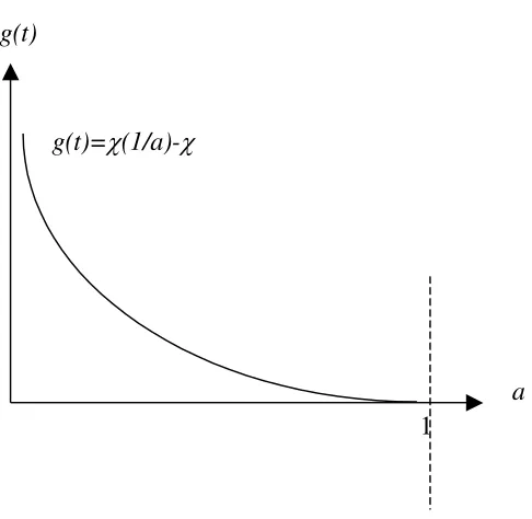
![Figure 11 shows the comparison between equations [18] and [16]](https://thumb-us.123doks.com/thumbv2/123dok_us/7853477.735897/78.595.92.447.74.460/figure-shows-comparison-equations.webp)