Soliton Solutions and Numerical Treatment of the Nonlinear Schrodinger’s Equation Using Modified Adomian Decomposition Method

(1)

http://www.scirp.org/journal/jamp ISSN Online: 2327-4379

ISSN Print: 2327-4352

Soliton Solutions and Numerical Treatment of the

Nonlinear Schrodinger’s Equation Using Modified

Adomian Decomposition Method

Abeer Al-Shareef1_{, Alyaa A. Al Qarni}2_{, Safa Al-Mohalbadi}1_{, Huda O. Bakodah}3

1_{Department of Mathematics, Faculty of Science, King Abdulaziz University, Jeddah, Kingdom of Saudi Arabia} 2_{Department of Mathematics, Faculty of Science, Blqarn Campus, Bisha University, Bisha, Kingdom of Saudi Arabia}

3_{Department of Mathematics, Faculty of Science, Al Faisaliah Campus, King Abdulaziz University, Jeddah, Kingdom of Saudi Arabia}

Abstract

In this paper, the improved Adomian decomposition method (ADM) is applied to the nonlinear Schrödinger’s equation (NLSE), one of the most important partial dif-ferential equations in quantum mechanics that governs the propagation of solitons through optical fibers. The performance and the accuracy of our improved method are supported by investigating several numerical examples that include initial condi-tions. The obtained results are compared with the exact solucondi-tions. It is shown that the method does not need linearization, weak or perturbation theory to obtain the solutions.

Keywords

Nonlinear Differential Equation, Schrödinger Equation, Adomian Decomposition, Reliable Technique

1. Introduction

The study of optical solitons has been going on for the past few decades [1]-[10]. The governing equation for the propagation of optical solitons for trans-continental and trans-oceanic distances through an optical fiber is given by the nonlinear Schrödinger’s equation (NLSE) that can be derived from the Maxwell’s equation with the aid of mul-tiple scale analysis. For birefringent fibers and dense wavelength division mulmul-tiplexed (DWDM) systems, this NLSE is generalized to the corresponding vector version. The scalar NLSE, with constant coefficients, which is typically used to study solitons in a polarization preserving fiber is integrable by the classical method of inverse scattering

How to cite this paper: Al-Shareef, A., Al Qarni, A.A., Al-Mohalbadi, S. and Bakodah, H.O. (2016) Soliton Solutions and Numeri-cal Treatment of the Nonlinear Schrodin-ger’s Equation Using Modified Adomian Decomposition Method. Journal of Applied Mathematics and Physics, 4, 2215-2232.

http://dx.doi.org/10.4236/jamp.2016.412215

Received: November 15, 2016 Accepted: December 23, 2016 Published: December 26, 2016

http://creativecommons.org/licenses/by/4.0/

(2)

transform (IST) and for Kerr law nonlinearity only. The NLS equation plays an impor-tant role in the modeling of several physical phenomena such as the propagation of optical pulses, waves in fluids and plasma, self-focusing effects in lasers, and trapping of atomic gas in Bose-Einstein condensates. Several numerical methods have been pro-posed to solve the nonlinear Schrödinger’s equation (NLSE) approximately. Many of them are explicit difference scheme [11][12] and Adomian decomposition method [13] [14] [15] [16] [17]. The Adomian decomposition method provides the solution in a rapid convergent series with computable terms. This method was successfully applied to nonlinear differential equations. Different modifications to solve nonlinear differen-tial equations are given in [18][19][20]. The modifications arise from evaluating diffi-culties specific for the type of problem under consideration. The modification usually involves only a slight change and is aimed at improving the convergence or accuracy of the solution. The main goal of this paper is to apply some modifications of Adomian decomposition method to the nonlinear Schrödinger’s equation and compare the re-sults with the exact solutions.

2. Analytical Solution for Nonlinear Schrodinger Equation (NLSE)

The dimensionless form of the generalized NLSE that is going to be studied in this pa-per is given by

( ) ( )

2

i m m m 0

t xx

u +β u +γ F u u =

Here, the dependent variable u is a complex valued function, while x and t are the two independent variables. The coefficients β and γ_{are constants and m is a}

con-stant parameter, where m≥1, transforms the NLSE to its generalized form. The

gene-ralized NLSE is partial differential equation that is not integrable, in general. The non- integrability is not necessarily related to the nonlinear term in it. Also, in generalized NLSE, F is a real-valued algebraic function and it is necessary to have the smoothness of the complex function 2

:

F u u C→C, considering the complex plane C as a two- dimensional linear space R2_{. The Kerr law of nonlinearity originates from the fact that a} light wave in an optical fiber faces nonlinear responses from non-harmonic motion of electrons bound in molecules, caused by an external electric field. Even though the nonlinear responses are extremely weak, their effects appear in various ways over long distance of propagation that is measured in terms of light wavelength. The origin of nonlinear response is related to the non-harmonic motion of bound electrons under the influence of an applied field. As a result the induced polarization is not linear in the electric field, but involves higher order terms in electric field amplitude. In the case of Kerr law nonlinearity where F u

( )

=u, thus the NLSE is given by

2

iut +uxx+γ u u=0 (2.1)

The aim of this section is to obtain an exact bright, dark, and singular 1-soliton solu-tion to this equasolu-tion. The Ansatz method is used. In order to set up the starting point, the solitons are written in the phase-amplitude format as

( )

( ),

, , ei x t

(3)

P is the amplitude component of the soliton and φ

( )

x t, is its phase component,

de-fined as φ

( )

x t, = − + +kx t θ. k is the frequency of the solution’s while ω represents

the wave number and θ is the phase constant. Substituting (2.2) and (2.3) into (2.1) and decomposing into real and imaginary parts lead to 2

(

2

)

3

1

2 0

P

P k P

x ω γ

∂ ₋ ₊ ₊ ₌

∂

and P k P 0

t γ x

∂ ₋ _⋅∂ ₌

∂ ∂ . From the imaginary part equation it is possible to obtain the

speed v of the soliton as v= −γk. The real part equation will be integrated from three types of solitons, namely, the bright, dark and singular soliton solution.

2.1. Bright Soliton

For bright solitons, the starting hypothesis is

sechp

P= A τ (2.2) and

(

–

)

B x vt

τ= (2.3) where, A represents the amplitude of the soliton and B is the inverse width of the soli-ton and v is the speed of the solisoli-ton.

(

2 2 2

)

2

(

)

2

(

3 3

)

sechp 1 sechp sech p 0

A ω+k −p B τ+ ⋅A pB p+ +τ γ− A τ = (2.4) Balancing principle yields

1

p= (2.5)

Substituting (2.5) into (2.4) we get

(

2 2

)

2 3

(

3 3

)

sech 2 sech sech 0

A ω+k −B τ+ A B⋅ τ γ− A τ = (2.6) Setting the coefficients of the linearly independent functions sechτ to zero leads to

(

2 2

)

.

B k

ω= − _{From coefficient} 3

sechτ we get ₂_B2₋γ_A2₌₀ and therefore

. 2

B= γA This leads to the bright soliton solution

( )

(

)

(- )

, sech ei kx t .

u x t =A _B x vt− _ + +ω θ

which will exist for the necessary constraints in place. 2.2. Dark Solitons

For dark solitons, the starting hypothesis is given by

tanhp

P= A τ (2.7) For dark solitons the parameters A and B are free parameters. Substituting and ap-plying Balancing principle yields

(

2 2

)

(

2 3

)

3

2 tanh 2 tanh 0

A ω+k + B τ− AB +γA τ = (2.8) From coefficient of the tanhτ into (2.8), we get 2 2

0

k B

ω + + = _{and therefore}

(

2 2

)

.

B k

ω= − − From coefficient of 3

tanh τ , we get 2 2

2B γA 0

(4)

. 2

B= −γ A This gives dark soliton solution u x t

( )

, =Atanh_B x vt

(

−

)

_ei(− + +kx ω θt )

along with their respective constraints as indicated. 2.3. Singular Solitons

For singular solitons, the starting hypothesis is given by cschp

P=A τ . Upon substi-tuting and applying balancing principle yields

(

2 2

)

(

2 3

)

3

csch 2 csch 0

A ω+k −B τ− AB +γA τ = (2.9) From coefficient of csechτ into (2.9), we get 2 2

0

k B

ω + − = _{and therefore}

(

2 2

)

.

B k

ω= − From coefficient of 3

cechτ, we get −₂_B2−γ_A2 =₀ and therefore

. 2

B= −γ A These lead to singular soliton solutions

( )

(

)

( )

, csch ei Kx t .

u x t =A _B x vt− _ − + +ω θ

which will exist for the necessary constraints in place.

3. Nonlinear Schrodinger Equation by Standard Adomian Method

(SADM)

The NLS equation describes the spatio-temporal evolution of the complex field

( )

,

u=u x t ∈C and has the general form (2.1) with the initial condition

( )

, 0

( )

u x = f x (3.1)

The solution of a nonlinear Schrödinger equation will be reduced by using standard Adomian decomposition method [21]. Equation (2.1) is rewritten in an operator form as

2

iLu+uxx+γ u ⋅u=0 (3.2)

where 1

( ) ( )

0 and . . d .

t

L L t

t

−

∂

= =

∂

∫

Then, the solution function, which obtains by Ado- mian decomposition method is assumed to be given by a series form

( )

0

, ,

n n

u x t u x t

∞

=

∑

_(3.3)

where the components un are going to be determined recurrently, while the nonlinear term is

( )

2

F u = u ⋅u in (2.1) is decomposed into an infinite series of polynomials of the form

( )

0

n n

F u A

= ∞

=

_∑

_(3.4)

The An called Adomian polynomials of u u0, ,1 un defined by

0 0

1

, 0,1, 2, 3 !

n

p

n n p

p d

A f u n

n d

λ λ λ

∞

= =

  

=    =

  

(5)

Operating on both sides of Equation (3.2) with the integral operator _L−1 after using

the initial displacements given by (3.1) and substituting Equations (3.3) and (3.4) into the resulting functional equation it gives

( )

2

( )

0 0 0

1

, i _n ,

n

n n

u x t f x L u x t A

x γ = = = ∞ ∞ ∞ −  ∂     = + _ _ _+ _ __ ∂      

∑

(3.6)

Then following the Adomian decomposition method introduced by Wazwaz [13] in order to solve Equation (3.6) the following recurrence relation is proposed

( )

(

)

( )

0

1 1 1

1 ,

, i i i , 0

xx xx

k k k k k

u x t f x

u₊ x t L− u γA L− u γL− A k

 =

 

= + = + ≥

 (3.7)

Setting 2 .

u =u u the Adomian polynomials A_k; k=0,1, 2, that represent the

nonlinear term F u

( )

.

4. The Modifications of the Adomian Decomposition Method

4.1. Reliable Technique

In this section, a reliable modification of the Adomian decomposition method de-composition method developed by Wazwaz [13] will be reduced. The modified form was established based on the assumption that the function f can be divided into two parts namely f0 and f1. Under this assumption we set f = f0+ f1.

Based on this, the modified recursive relation is formulated as follows

( )

0 0

1 1

1 1 0 0

1 1

1

i i

i i 1

xx

n k k

u f

u f L u L A

u L u L A n

γ γ − − − − +  =   = + +   = + ≥  (4.1)

The choice of f0 and f1 such that uk contains the minimal number of terms has a strong influence accelerates the convergence of the solution. The modification demonstrate a rapid convergence of the series solution if compared with standard (ADM) and it may give the exact solution for nonlinear equations by using two itera-tions only without using the so-called Adomian polynomials.

4.2. The New Modification

In the new modification [22], Wazwaz replaced the process of dividing f into two com-ponent by a series of infinite comcom-ponents, so f be expressed in Taylor series

( )

n 0 n

f x =

∑

∞= f . Moreover, he suggests a new recursive relationship expressed in the form

( )

0 0

1 1

1 i _xx i 0

n n k k

u f

u+ f L− u γL− A n

= 

 ₌ ₊ ₊ _≥

 (4.2)

(6)

the modified relation (4.1).

5. Numerical Illustrations

5.1. Example 1

Consider the nonlinear cubic Schrodinger equation (NLS) which has the general form

2

0 1 0

2

i u u q u u 0; L x L t, ,t

t x

∂ ₊∂ ₊ ₌ _{< <} _>

∂ ∂ (5.1)

where q≥0 is a real parameter and. In Equation (2.12) the function u governs the

evolution of a weakly nonlinear, strongly dispersive, almost monochromatic wave. As-suming initial condition of the form,

(

, 0

)

( )

u x t = f x (5.2)

and boundary conditions

(

0

)

(

1

)

0

, ,

0; ,

u L t u L t

t t

x x

∂ ∂

= = ≥

∂ ∂ (5.3)

the initial boundary value problem (IBVP) (5.1)-(5.3) gives rise to soliton solutions in which the solution and its derivatives with respect to x vanish as x → ∞ [23][24].

For the single-soliton case, when q≠0, the function

( )

(

)

1 1 2 2 2 1

, exp sech ,

2

a

u x t i cx t a x ct

q θ        =   _ − _  −     

    (5.4)

where 2

4 ,

c a

θ = − satisfies Equations (2.12)-(2.14). For fixed t the function u in Eq-uation (5.4) decays exponentially as x → ∞ and it represents a soliton-type

distur-bance which travels with speed c; its amplitude is governed by the real parameter a. 1) Standard Adomian Decomposition Method

Consider the initial condition

( )

1 1 2 2 2 1

, 0 exp sech ,

2

a

u x i cx a x

q        =_ _ _ _ __ _ _    

    (5.6)

Using standard ADM the solution of the NLS equation is given by the following ap-proximation;

( )

(

)

(

)

(

)

(

)

(

)

1 1 2 2 0 1 2 3 2 1

, exp s ech ,

2

,

0.002828427i sech 0.1 cos 0.05 i sin 0.05 cos 0.05 i sin 0.05 a

u x t i cx a x

q

u x t

t x x x x x

       =   _ _           = − +

The approximating Adomian decomposition method was tested to NLS equation for the single-soliton wave to the problems with boundary lines L0 = −80 and L1= −80.

In Figure 1 it is presented the modulus u _{of the theoretical solution of NLS with q =}

(7)

[image:7.595.198.550.71.364.2]

Figure 1. The graph of the exact solution for example 1.

[image:7.595.197.547.397.687.2]

(8)

2) Reliable Technique

Now we assume that the function f can be divided into two parts namely f0 and 1

f . Under this assumption we set

( )

1 1 2 2 0 1 1 2 2 1 0 0 1 0 2 1

, cos sech ,

2

2 1

, i sin sech i d

2 , i d , 1

t

n n

a

u x t cx a x

q

a

u x t cx a x q A t

q

u + x t q A t n

      =_ _ _ _ _ _             =_ _ _ _ _ _+       = ≥

∫

[image:8.595.193.553.294.482.2]

In Table 2 various time step combinations are examined and compared with results given by exact solution.

Table 1. The absolute error when x = 10.

[image:8.595.194.554.514.701.2]

Standard ADM T 0.0000703381 0.1 0.000140626 0.2 0.000210864 0.3 0.000281052 0.4 0.00035119 0.5 0.000421277 0.6 0.000491314 0.7 0.0005613 0.8 0.000631235 0.9 0.00070112 1.0

(9)

3) The New Modification

In the new modification, the process of dividing f into two components is replaced by a series of infinite components. The recursive relationship expressed in the form

( )

0

1 0

0

2 2

0 , 0.1414213,

, 0.00707106i i d

, 0.00088388 i d ,

t

n

u x t

u x t x q A t

u x t x q A t

=

= +

∫

Remark. When using the new modification for ADM the computations of the inte-grals will be simpler but we need a large number of components to get accurate results, which may lead to accumulation of round of error.

5.2. Example 2

Consider the nonlinear Schrodinger equation (NLS)

2

2 2

i u u 2u u 0

t x

∂ ₊∂ ₊ ₌

∂ ∂ (5.7)

Subject to the initial condition of the form,

( , 0) eix

u x = (5.8)

1) The Standard ADM

So, we get the recurrent relation

( )

0 , e

ix u x t =

( )

1 1

1 , i _xx 2i

k k k

u + x t = L u− + L A−

We can calculate few terms as

( )

1 1 1

( )

1

( )

1 , i 0xx 2i 0 e 2i e i e

ix ix ix

u x t = L u− + L A L− − − + L− = t

( )

1 1

2 , i 1xx 2i 1

u x t = L u− + L A−

The solution is

( )

2 3

0 1 2 3 0

1 1

, e i e e i e

2 3!

ix i ix ix

n

x n

u x t u u u u t t t

∞

=

= + + + = + − − +

∑

 

The behavior of the ADM solution obtained for different values of time is compared with the exact solution in Figure 3. It is to be noted that the exact solution of u x t

( )

,

was given as u x t

( )

, =ei x t( +).

In Table 3, the absolute errors in different time value are listed.

Remark: As it seen from Figure 3, the numerical results of ADM are in very good agreement with their analytical values obtained from the exact solution. Moreover, from Figure 4 it can be seen that the error are somewhat small as the number of the components (n) in Adomian series is increasing.

(10)

[image:10.595.45.561.61.181.2]

t = 0.1 t = 0.3 t = 0.5 Figure 3. The graph of the exact solution and ADM solution at t = 0.1, t = 0.03 and t = 0.5.

Table 3. The absolute error when t = 0.03, t = 0.1 and t = 0.5.

x Absolute Error at t = 0.03 Absolute Error at t = 0.1 Absolute Error at t = 0.5

0 3.370059347 × 10−8 _{0.0000041661332570} _0.0025955039

0.1 3.370059347 × 10−8 _{0.0000041660562770} _0.0025955040

0.2 3.381153649 × 10−8 _{0.0000041661206330} _0.0025955039

0.3 3.374685170 × 10−8 _{0.0000041660544070} _0.0025955038

0.4 3.377217790 × 10−8 _{0.0000041660937870} _0.0025955040

0.5 3.379127106 × 10−8 _{0.0000041661050360} _0.0025955038

0.6 3.370356064 × 10−8 _{0.0000041660713930} _0.0025955040

0.7 3.375440712 × 10−8 _{0.0000041660511770} _0.0025955038

0.8 3.373499667 × 10−8 _{0.0000041662206490} _0.0025955036

0.9 3.376684765 × 10−8 _{0.0000041661306230} _0.0025955037

1.0 3.370830758 × 10−8 _{0.0000041660782630} _0.0025955036

[image:10.595.40.554.229.589.2]

n = 1 n = 2 n = 3 Figure 4. The graph of the exact solution and ADM solution at n = 1, n = 2 and n = 3.

We set

( )

0

1 0 0

0 0

1

0 0

, Cos

, iSin i d i d

, i d i d , 1

t t

xx

t t

n n xx n

u x t x

u x t x u t q A t

u₊ x t u t q A t n

=

= + +

= + ≥

∫

(11)

In Table 4, various time step combinations are examined and compared with exact solution.

[image:11.595.182.539.82.409.2] [image:11.595.198.487.192.387.2]

The behavior of the Reliable ADM solution is compared with the exact solution in

Figure 5.

3) The New Modification

To apply the new modification we replace f by a series of infinite components. Then, we can calculate few terms as

0 0 1

u = f =

( )

1

1 1 i 0xx 2i 0 i 2i .

u = f + L− u + A = +x t

( )

2

1 2

2 2 i 1 2i 1 2 2 .

2

xx

x

u = f + L− u + A = − − xt− t

( )

3

1 2 2 3

3 3 2 2

4

i 2i i i i 2i i .

6 3

xx

x

u = f + L− u + A = − − −t x t− xt − t

where

2

2 0 1, 1 i 2i 2 2 2 ,

2 x

A = A = +x tA = − − xt− t 

The solution is

2 3

2 2 2 4 3

i 2i 2 2 i i i 2i i

2 6 3

x x

u= +x t− − xt− t − − −t x t− xt − t +

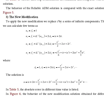
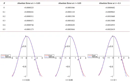
In Table 5, the absolute error in different time value is listed.

[image:11.595.48.555.454.689.2]

In Figure 6, the behavior of the new modification solution obtained for different values of time:

Reliable ADM

T

0.257913922 0.1

0.0448678059 0.2

0.0584708828 0.3

0.0687497541 0.4

0.079066386 0.5

(12)

[image:12.595.43.554.86.407.2]

Table 5. The absolute error when t = 0.03, t = 0.05 and t = 0.1.

X Absolute Error at t = 0.03 Absolute Error at t = 0.05 Absolute Error at t = 0.1

0 +0.0000225 +0.0001046 +0.0008482

0.1 +0.0000241 +0.0001110 +0.0009063

0.2 +0.0000311 +0.0001338 +0.0010460

0.3 +0.0000471 +0.0001822 +0.0013000

0.4 +0.0000746 +0.0002630 +0.0016955

[image:12.595.42.553.90.407.2]

0.5 +0.0001173 +0.0003844 +0.0022619

Figure 6. The graph of the exact solution and new modification solution at t = 0.03, t = 0.05 and t = 0.1

6. The Improved Adomian Decomposition Method

6.1. The Method

In our new calculation, the complex system given in Equation (1) in converted into a real system by writing

( )

, 1 i 2

u x t =q + q (6.1)

where

(

q k_k, =1, 2

)

are real functions. By substituting Equation (6.1) into Equation (2.1), we obtain the following system

(

2 2

)

1t 2xx 1 2 2 0

q +q +γ_ q +q _q = (6.2)

(

2 2

)

2t 1xx 1 2 1 0

q −q −γ_ q +q _q = (6.3)

where q x1

( )

,0 = u x

( )

,0 _R,q x2

( )

,0 = u x

( )

,0 _I In an operator form, Equations (6.2) and

(6.3) become

( )

(

2 2

)

1 2 1 2 2 0 t xx

L q +q +γ_ q +q _q = (6.4)

( )

(

2 2

)

2 1 1 2 1 0 t xx

L q −q −γ_ q +q _q = (6.5)

Applying the inverse operator 1 t

(13)

( )

1 1 1 , 1 ,0 2xx 1

q x t =q x −L q− −L A− (6.6)

( )

1 1

2 , 2 , 0 1xx 2

q x t =q x +L q− +L A− (6.7) Assumes that, the nonlinear terms in (6.6) and (6.7) are represented by the following series

(

2 2

)

1 1 2 2 2

A =_γ q +q _q =Sq (6.8)

(

2 2

)

2 1 2 1 1

A =_γ q +q _q =Sq (6.9)

1, 2

A A are Adomian polynomials. Substituting the nonlinear terms (6.8) and (6.9) and the solution form (6.4) and (6.3) into (6.6) and (6.7) gives

( )

1 1

1

0 0 0

1 2 1

, , 0 ( ( , ))

n n

n xx n

n

q x t q x L q x t L A

∞ ∞ ∞ = − = − = = − −

∑

(6.10)

( )

1 1

2

0 0 0

2 1 2

, , 0 ( ( , ))

n n

n xx n

n

q x t q x L q x t L A

∞ ∞ ∞ = − = − = = + +

∑

(6.11)

Following the decomposition analysis, we introduce the recursive relative

( )

1,0 , 1 , 0

q x t =q x (6.12)

( )

2,0 , 2 , 0

q x t =q x (6.13)

( )

1

(

( )

)

1

1,k 1 , 2,k , _xx 1,m

q + x t = −L− q x t −L A− (6.14)

( )

1

(

( )

)

1

2,k 1 , 1,k , _xx 2,m

q + x t = +L− q x t +L A− (6.15) Adomian polynomials are calculated as follows

(

)

(

2 2

)

1,0 1,0 2,0 2,0.

A = γ q +q q (6.16)

(

)

(

)

(

2 2

)

1,1 2 1,0 1,1 2 2,0 2,1 2,0 1,0 2,0 2,1.

A = γ q q + q q q + γ q +q q (6.17)

(

)

(

)

(

)

(

) (

)

(

)

2 2

1,2 1,0 1,2 1,1 2,0 2,2 2,1 1,0 1,1 2,0 2,1

2 2 2 2

1,0 2,0 1 3,0 4,0 2,2

1

4 2 4 2 2

2

.

A q q q q q q q q q q

q q c q q q

γ γ

γ

= + + + + +

+ + + + (6.18)

Similarly we can calculate A2,0, A2,1,. Now, the first components from Equations

(6.12)-(6.15) can be determined. Substituting these values into Equations (6.2) and (6.3), we can obtain the expression of q1 and q2, the closed form solutions yield from

Equ-ations (6.1).

6.2. Test Problems

The method is applied to the two above examples. 1) Solution of Example 5.1 with IADM

(14)

(

2 2

)

1t 2xx 2 1 2 2 0

q +q + q +q q =

(

2 2

)

2t 1xx 2 1 2 1 0

q q q q q

− + + + =

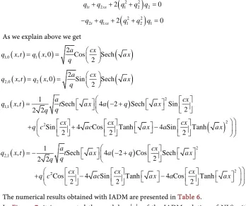
As we explain above we get

( )

1,0 1

2

, , 0 Cos Sech

2

a cx

q x t q x a x

q   = = _ _  

( )

2,0 2 2

, , 0 Sin Sech

2

a cx

q x t q x a x

q   = = _ _  

( )

(

)

( )

2 1,1 2 2 1

, Sech 4 2 Sech Sin

2 2 2

Sin 4 Cos Tanh 4 Sin Tanh

2 2 2

a cx

q x t t a x a q a x

q q

cx cx cx

q c ac a x a a x

       = _ __ − + _ _ _{ }          _ _    + _  _{ }+  _{ }  −  _{ } _

( )

(

)

2

2,1

2 2

1

, Sech 4 2 Cos Sech

2 2 2

Cos 4 Sin Tanh 4 Cos Tanh

2 2 2

a cx

q x t t a x a q a x

q q

cx cx cx

q c ac a x a a x

       = − _ __ − + _{ } _ _          _ _   _ _  + _ _{ } − _{ }   −  _{ }   _

The numerical results obtained with IADM are presented in Table 6.

In Figure 7, it is presented the modulus u of the IADM solution of NLS with 1, 0.01

q= a= and velocity c=0.1 for t∈

[

0,180

]

.

2) Solution of Example 5.2 with IADM We consider following Schrodinger equation

2

iut+uxx+2u u=0 (6.19)

With initial and boundary condition

( )

, 0 eix

u x = . This problem has an exact solu-tion u x t

( )

, =ei x t( +) In our calculation, we will convert the complex equation given in

Equation (6.19) into a real system by writing

(

2 2

)

1t 2xx 2 1 2 2 0

q +q + q +q q =

(

2 2

)

2t 1xx 2 1 2 1 0

q q q q q

− + + + =

[image:14.595.199.548.74.366.2]

As is explained above, the iterative relation is obtained as

Improve ADM

T

4.6052711 × 10−8

0.1

1.8421550 × 10−7

0.2

4.1449535 × 10−7

0.3

7.3689919 × 10−7

0.4

(15)

[image:15.595.201.545.71.313.2]

Figure 7. The graph of the approximate solution (IADM) for example 1.

( )

1,0 , 1 , 0 cos

q x t =q x = x (6.20)

( )

2,0 , 2 , 0 sin

q x t =q x = x (6.21)

( )

1

( )

1

1,k 1 , t 2,k _xx 2 t 1,k

q ₊ x t = −L− q − L A− (6.22)

( )

1

( )

1

2,k 1 , t 1,k _xx 2 t 2,k

q + x t =L− q + L A− (6.23) Adomian polynomials are calculated as follows

2 3

1,0 1,0 2,0 2,0.

A =q q +q

2 2

1,1 1,0 2,1 2 1,0 1,1 2,0 3 2,0 2,1.

A =q q + q q q + q q

2 2 2 2

1,2 1,0 2,2 2 1,0 1,1 2,1 2 1,0 1,2 2,0 1,1 2,0 3 2,0 2,2 3 2,1 2,0.

A =q q + q q q + q q q +q q + q q + q q

Similarly we can calculate A2,0, A2,1. Now, the first components can be determined.

( )

1,0 , 1 , 0 cos

q x t =q x = x

( )

2,0 , 2 , 0 sin

q x t =q x = x

( )

1,1 , Sin

q x t = −t x

( )

2,1 , Cos

q x t =t x

( )

2

( )

1,2

1

, Cos

2

q x t = − t x

( )

2

( )

2,2

1

, Sin

2

q x t = − t x

(16)

[image:16.595.191.553.89.192.2]

Improve ADM

T

1.6680003 × 10−7

0.1

0.000005331568 0.2

0.0000404691114 0.3

0.0001704381222 0.4

0.0005197377272 0.5

7. Conclusion

In this work, it is shown how the Adomian decomposition method and some of its modification can be adapted in order to be used to the nonlinear Schrodinger. The new method presented in this work has a powerful and easy use. The numerical technique is improved by decomposition of the nonlinear operator. In applying the improved Ado-mian decomposition Method (IADM) to the nonlinear Schrodinger equation, it is found that the method gives accurate results with lesser computational effort as com-pared with other modification.

Conflict of Interest

The authors declare that there is no conflict of interest regarding the publication of this paper.

References

[1] Eslami, M., Mirzazadeh, M., Vajargah, B.F. and Biswas, A. (2014) Optical Solitons for the Resonant Nonlinear Schrödinger’s Equation with Time-Dependent Coefficients by the First Integral Method. Optik—International Journal for Light and Electron Optics, 125, 3107- 3116. https://doi.org/10.1016/j.ijleo.2014.01.013

[2] Crutcher, S.H., Osei, A.J. and Biswas, A. (2013) Wobbling Phenomena with Logarithmic Law Nonlinear Schrödinger Equations for Incoherent Spatial Gaussons. Optik—International Journal for Light and Electron Optics, 124, 4793-4797.

https://doi.org/10.1016/j.ijleo.2013.01.081

[3] Triki, H., Hayat, T., Aldossary, O.M. and Biswas, A. (2012) Bright and Dark Solitons for the Resonant Nonlinear Schrödinger’s Equation with Time-Dependent Coefficients. Optics & Laser Technology, 44, 2223-2231. https://doi.org/10.1016/j.optlastec.2012.01.037

[4] Biswas, A. and Milovic, D. (2009) Travelling Wave Solutions of the Non-Linear Schrödin-ger’s Equation in Non-Kerr Law Media. Communications in Nonlinear Science and Nu-merical Simulation, 14, 1993-1998. https://doi.org/10.1016/j.cnsns.2008.04.017

[5] Lott, D.A., Henriquez, A., Sturdevant, B.J.M. and Biswas, A. (2009) A Numerical Study of Optical Soliton-Like Structures Resulting from the Nonlinear Schrödinger’s Equation with Square-Root Law Nonlinearity. Mathematics and Computation, 207, 319-326.

https://doi.org/10.1016/j.amc.2008.10.038

(17)

4246-4256. https://doi.org/10.1016/j.ijleo.2014.04.014

[7] Masemola, P., Kara, A.H. and Biswas, A. (2013) Optical Solitons and Conservation Laws for Driven Nonlinear Schrödinger’s Equation with Linear Attenuation and Detuning. Optics & Laser Technology, 45, 402-405. https://doi.org/10.1016/j.optlastec.2012.06.017

[8] Biswas, A., Moran, A., Milovic, D., Majid, F. and Biswas, K.C. (2010) An Exact Solution for the Modified Nonlinear Schrödinger’s Equation for Davydov Solitons in α-Helix Proteins. Mathematical Biosciences, 227, 68-71. https://doi.org/10.1016/j.mbs.2010.05.008

[9] Biswas, A. and Milovic, D. (2010) Bright and Dark Solitons of the Generalized Nonlinear Schrödinger’s Equation. Communications in Nonlinear Science and Numerical Simulation, 15, 1473-1484. https://doi.org/10.1016/j.cnsns.2009.06.017

[10] Biswas, A (2009) 1-Soliton Solution of 1 + 2 Dimensional Nonlinear Schrödinger’s Equa-tion in Power Law Media. Communications in Nonlinear Science and Numerical Simula-tion, 14, 1830-1833. https://doi.org/10.1016/j.cnsns.2008.08.003

[11] Weizhong, D. (1992) An Unconditionally Stability Three-Level Explicit Difference Scheme for the Schrödinger Equation with a Variable Coefficient. SIAM Journal on Numerical Analysis, 29, 174-181. https://doi.org/10.1137/0729011

[12] Chan, I.T.E, Lee, D. and Shen, L. (1986) Stable Explicit Scheme for Equation of the Schrödinger Type. SIAM Journal on Numerical Analysis, 23, 274-281.

https://doi.org/10.1137/0723019

[13] Wazwaz, A.M. (2001) A Reliable Technique for Solving Linear and Nonlinear Schrodinger Equations by Adomian Decomposition Method. Bulletin of the Institute of Mathematics Academia Sinica, 29, 125-134.

[14] Sadighi, A. and Ganji, D.D. (2008) Analytic Treatment of Linear and Nonlinear Schrödin-ger Equations: A Study with Homotopy-Perturbation and Adomian Decomposition Me-thods. Physics Letters A, 372, 465-469. https://doi.org/10.1016/j.physleta.2007.07.065

[15] Mezban, M.O. and Shnnan, A.K. (2009) Adomian’s Decomposition Method for Solving One Dimensional Schrödinger Equation. Journal of Basrah Researches (Sciences), 35, 5-11. [16] Kumar, A. and Pankaj, R.D. (2013) Solitary Wave Solutions of Schrödinger Equation by

Laplace-Adomian Decomposition Method. Physical Review & Research International, 3, 702-712.

[17] Maitama, S. (2014) A New Approach to Linear and Nonlinear Schrodinger Equations Using the Natural Decomposition Method. International Mathematical Forum, 9, 835-847. [18] Wazwaz, A.M. (1999) The Modified Decomposition Method and Padé Approximants for

Solving the Thomas-Fermi Equation. Applied Mathematics and Computation, 105, 11-19.

https://doi.org/10.1016/S0096-3003(98)10090-5

[19] Wazwaz, A.M. (1999) A Reliable Modification of Adomian Decomposition Method. Ap-plied Mathematics and Computation, 102, 77-86.

https://doi.org/10.1016/S0096-3003(98)10024-3

[20] Wazwaz, A.M. (2005) Adomian Decomposition Method for a Reliable Treatment of the Edman-Flower Equation. Applied Mathematics and Computation, 161, 543-560.

https://doi.org/10.1016/j.amc.2003.12.048

[21] Adomian, G. and Rach, R. (1991) Linear and Nonlinear Schrödinger Equations. Founda-tions of Physics, 21, 983-991.

(18)

[23] Argyris, J. and Haase, M. (1987) An Engineer’s Guide to Soliton Phenomena: Application of the Finite Element Method. Computer Methods in Applied Mechanics and Engineering, 61, 71-122. https://doi.org/10.1016/0045-7825(87)90117-4

[24] Sanz-Serna, J.M. (1986) Conservative and Nonconservative Schemes for the Solution of the Non-Linear Schrodinger Equation. IMA Journal of Numerical Analysis, 6, 25-42.

https://doi.org/10.1093/imanum/6.1.25

Submit or recommend next manuscript to SCIRP and we will provide best service for you:

Accepting pre-submission inquiries through Email, Facebook, LinkedIn, Twitter, etc. A wide selection of journals (inclusive of 9 subjects, more than 200 journals)

Providing 24-hour high-quality service User-friendly online submission system Fair and swift peer-review system

Efficient typesetting and proofreading procedure

Display of the result of downloads and visits, as well as the number of cited articles Maximum dissemination of your research work

Submit your manuscript at: http://papersubmission.scirp.org/