Market risk of developed and developing countries during the global financial crisis

Munich Personal RePEc Archive

Market risk of developed and developing

countries during the global financial crisis

Köksal, Bülent and Orhan, Mehmet

Central Bank of Turkey, Fatih University - Department of Economics

March 2012

Online at

https://mpra.ub.uni-muenchen.de/37523/

Market Risk of Developed and Developing Countries

During the Global Financial Crisis

Bülent Köksal † and Mehmet Orhan ‡ March 2012

Abstract: This study compares the performance of the widely used risk measure Value-at-Risk (VaR) across a large sample of developed and developing countries. The performance of the VaR is assessed by both unconditional and conditional tests of Kupiec and Christoffersen, respectively, as well as the Quadratic Loss Function. Results indicate that the performance of VaR as a measure of risk is much worse for developed countries than the developing ones during our sample period. One possible reason might be the deeper initial impact of global financial crisis on developed countries than emerging markets. Results also provide evidence of decoupling between emerging and developed countries in terms of market risk during the global financial crisis.

JEL Classification Codes: C32; C51; G01; G32.

Keywords: Value-at-Risk (VaR), Developed Countries, Emerging Markets, ARCH/GARCH Estimation, Kupiec Test, Christoffersen Test, Quadratic Loss Function.

* _{The views expressed in this paper belong to the authors and do not necessarily represent those of the Central}

Bank of Turkey or its staff.

† _{Corresponding author, Central Bank of Turkey, Istiklal Cad. 10, Ulus, 06100 Ankara, Turkey.}

Tel: +90 312 507 5899. E-mail: bulent.koksal@tcmb.gov.tr.

‡ _{Department of Economics, Fatih University, Istanbul, Turkey. Tel: +90 212 866 33 00, Ext: 5012.}

1

1.

Introduction

Risk management has become even more crucial after the 2007-2009 global financial crisis

that hit the world economy.1 The risk will be reflected in the risk premium which is determined by the repayment capability of the borrower. Each borrower has to pay the “risk

premium” based on his perceived risk. It is surprising to note that several developed countries

are influenced from the crisis more adversely than the emerging market economies as

reflected by the Credit Default Swap (CDS) rates (see Figure 1).

[Insert Figure 1]

It is interesting that the firms with expertise in risk management have collapsed while or after

the global financial crisis.2 Mismanaged risk together with technological advances in the financial sector contributed to the global financial crisis. A special report published by the

European Commission (2009) that examines the anatomy of the crisis states that “The crisis

was preceded by long period of rapid credit growth, low risk premiums, abundant availability

of liquidity, strong leveraging, soaring asset prices and the development of bubbles in the real

estate sector. Over-stretched leveraging positions rendered financial institutions extremely

vulnerable to corrections in asset markets. As a result a turn-around in a relatively small

corner of the financial system (the US subprime market) was sufficient to topple the whole

structure.” Many of the countries had to support their financial intermediaries because of the

toxic assets in their balance sheets with significantly lower values.3 The cost of dealing with the consequences of the crisis created huge budget deficits and contributed to the low

economic growth not only in small EU countries like Greece, Ireland, but also in more

1 _{For an analysis of the crisis with respect to its different dimensions, see the special issues of the Journal of}

International Money and Finance (Volume 28, Issue 8, 2009) on “The Global Financial Crisis: Causes, Threats and Opportunities”, the Journal of International Economics on “The Global Dimensions of the Financial Crisis” (forthcoming) and the Journal of Asian Economics (Volume 21, Issue 3, 2010) on “The Financial Crisis of 2008-09: Origins, Issues, and Prospects”.

2 _{For a list of acquired or bankrupt banks in the 2007-2009 global financial crisis, see}

http://en.wikipedia.org/wiki/List_of_acquired_or_bankrupt_banks_in_the_late_2000s_financial_crisis (retrieved on March 20, 2012). See Tett (2009) for a detailed overview of AIG’s collapse.

2

advanced economies like Spain, Italy and the UK. Basel II Accord provided guidelines in

terms of capital requirements for a sound banking system but it was heavily criticized for

boosting procyclicality of the banking sector.4 In response, the Basel Committee on Banking Supervision established revised global standards, known as Basel III.

VaR (Value-at-Risk) is devised as unit free risk measure which is very convenient for practical

purposes. In its simplest form it is defined as the maximum expected loss of a portfolio at the

given confidence level and holding period. VaR became more popular especially due to its

simplicity (Giot and Laurent (2004)). As Berkowitz and O’Brien (2002) put “Value-at-Risk

has become a standard measure of financial market risk that is increasingly used by other

financial and even non-financial firms as well.” Its popularity increased after Bank for

International Settlements and SEC address VaR as a measure to quantify risk as well as Basel

Committee on Banking Supervision’s (1994, 1996) imposition of VaR use on financial

institutions. The use of VaR in assessing risk is not limited to financial markets only. Giot and

Laurent (2003), for instance, make use of ARCH to calculate VaR in commodities markets of

aluminum, copper, nickel, and Brent crude oil. Naïve methods like variance-covariance and

historical simulation could not survive because of their considerable shortcomings and there is

a remarkable progress in computing more accurate VaR but in the expense of more

complicated and sophisticated computation techniques that require more effort and time.

Advances in the information technology enabled investors to perform VaR estimations that

were not possible two decades ago.

This study compares the performance of the widely used Value-at-Risk (VaR) across a large

sample of countries and provides evidence of decoupling between emerging and developed

4 _{See Cannata and Quagliariello (2009) and Moosa (2010) for discussions. Goodhart (2008) describes the}

3

countries in terms of market risk during the global financial crisis. Current literature about the

decoupling finds that emerging countries were isolated from the developments in the U.S.

financial markets at the beginning of the crisis but followed the rest of the developed

countries afterwards in terms of their reaction to the worsening situation in the U.S.

economy.5 Our study contributes to this literature by providing evidence of decoupling from the perspective of Value-at-Risk.

The rest of the paper is organized as follows. Section 2 describes empirical methodology and

data. Section 3 describes the tests to evaluate VaR and discusses the results while Section 4

concludes.

2.

Empirical Methodology and Data

VaR is the maximum expected percentage loss possible at a given confidence level for some

specified investment horizon. More technically, VaR (1−α) is defined as the threshold that is

exceeded 100*α times out of 100 trials on average. 1−α is the confidence level where α ∈

(0,1) is a real number. The cases where ex-post portfolio returns are lower than VaR estimates

are called violations. One main input to the VaR calculation is the confidence level, (1−α ).

Once the confidence level is set, VaR must be calculated in such a way that the violations

should be equal to 100*α . For instance, if one wants to have the 95% confidence level, then

VaR must be computed in such a way that the loss worse than the VaR will be 5% of all cases

on average. That is, percentage of the losses greater than the suggested VaR will be 5 times

out of every 100 cases on average. Therefore, VaR is the unique number based on the time

series under focus.

5 _{See Akın and Kose (2008), Dooley and Hutchison (2009), Felices and Wieladek (2012), Fidrmuc and Korhonen}

4

The second input that is necessary to calculate VaR is the standard deviation or volatility of

the returns. Modeling and forecasting volatility is crucial for investors who are interested in

the forecast of the variance of a time-varying portfolio return over the holding period to

calculate VaR. The long-run forecast of the unconditional variance would be irrelevant for

these investors who hold the asset for a certain period only. In a seminal paper, Engle (1982)

shows how to model the conditional variance of a time series. Bollerslev (1986) generalizes

Engle’s work by allowing the conditional variance to be an ARMA process. These models are

called GARCH (Generalized Autoregressive Conditional Heteroskedasticity) models.6 Most recent and advanced VaR methods make use of GARCH models to calculate the conditional

standard deviation.7

One issue that has to be addressed is to determine the specific GARCH model to estimate the

conditional standard deviation since there have been quite a few models discussed in the

literature. In his “Glossary to ARCH (GARCH)”, Bollerslev (2008) lists more than 100

entries. In a related work, Orhan and Köksal (2012) compare the performances of 16 different

GARCH specifications for calculating VaR using the same data and sample period as the ones

used in this study. Accordingly, we use the conditional variance model selected by that study

as the best model which is the simple ARCH model with one lag where the errors follow the t

distribution.8 Specifically, our model for calculating the conditional variance (and standard deviation) is as follows:

t t t

r = +µ ε

0 1 1

t t

µ β β ε= + −

6 _{See Poon and Granger (2003) for an extensive survey.}

7 _{See, for example, Angelidis et al (2004), Ane (2006), Hartz et al (2006), and Fan et al (2008).}

8 _{GARCH model likelihoods are notoriously difficult to maximize. ARCH(1) model has the additional benefit of}

5

t t tv

ε σ=

2 1

( |t t ) t

Var ε I₋ =σ

2 2

1 1

t t

σ = +ω α ε₋

where rt =ln(pt / pt−₁), pt being the closing price of a country index (as described in the next

section) at the end of day t, µt =E r I( |t t−1) is the conditional mean, It−1 denotes the

information set available at time t-1 and vt is a sequence of i.i.d. random variables with mean

0 and variance 1. We assume that vt follow the standardized Student-t distribution which

appropriately deals with the issue of fat tails of returns documented in the financial literature.

In this setting VaR is defined as:

Pr(rt <VaR(1−α))=α

Once the conditional variance terms, σˆ_t2, are estimated, VaR is defined as:

ˆ

(1 ) t

VaR −α = −r σt_α

where r is the mean return, and t_α is the critical value of the t distribution with right-tail area

α .

Although there are papers in the literature that calculate the VaR by utilizing GARCH models,

to the best of our knowledge, this is the first study that compares the performance of VaR

across a large sample of developed and emerging market economies by using data from the

6

We make use of the country indices for 44 developed and emerging market countries obtained

from MSCI website.9 This website describes the construction of the indices as “To construct a country index, every listed security in the market is identified. Securities are free float

adjusted, classified in accordance with the Global Industry Classification Standard (GICS®),

and screened by size, liquidity and minimum free float.” For each country, we use a total

number of 1887 daily returns starting from May 30th, 2002 to August 24, 2009 to estimate the conditional standard deviations for VaR calculations using a 1000-day rolling window.

Because of the rolling-window methodology that we employ, our final sample includes 888

estimated values of conditional standard deviations for the period March 30th, 2006 - August

24, 2009 which overlaps with the global financial crisis.10 We calculate both in-sample and out-of-sample comparisons but report only the out-of-sample figures as the in-sample results

are similar.

3.

VaR as a Measure to Assess Market Risk

Basel Committee on Banking and Supervision asked for the implementation of VaR as well as

the out-of-sample backtesting (Escanciano and Olmo (2011)). There are basically two

approaches that use back-testing to compare the performance of VaR calculations in the

finance literature. The “unconditional” approach does not take the sequence of violations into

account. Using this approach, Kupiec (1995) defines the following test statistic that follows

the χ2 Distribution with 1 degree of freedom:

(

)

( )

(

)

F F N N F N F

K

α

α

− − −                     −

=2ln 1 2ln 1

7

where N is the total number of trials and F is the number of violations. If a method is perfect

in returning the VaR figures, (F/N) will converge to α as suggested by the null hypothesis,

0

H , and K will be approximately zero. In the opposite case, the difference between

percentage of violations and α will be larger causing the test statistic to increase which

means that the likelihood of null’s rejection will be higher.11 Kupiec Test assumes that the number of failures, F, follows the Binomial Distribution with parameters N and α. Based on

the selected level of α , rejection of the Kupiec test’s null hypothesis for a country implies

that VaR is not very useful as a measure of market risk for that country.

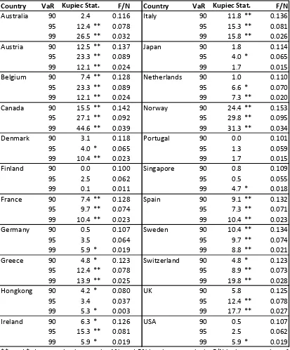
Table 1, Panel A reports the Kupiec Test statistics for 5% and 1% significance levels as well

as the proportion of violations for developed countries. Ideally, the proportion of violations

should be approximately 0.1, 0.05, and 0.01, for VaR with 90%, 95%, and 99% confidence

levels, respectively, and the Kupiec Test statistic should be close to 0. Panel B reports the

number of rejections and non-rejections. Overall conclusion from Panel B is that # of

rejections is much larger than the number of non-rejections implying that VaR as a measure of

risk was not successful for developed countries during the crisis period.

[Insert Table 1]

The VaR methodology performed poorly particularly in Austria, Belgium, Canada, France,

Italy, Norway, Spain and Sweden where the null hypothesis of the Kupiec test was rejected at

all 90%, 95%, and 99% VaR confidence levels. VaR was a good measure of risk for Portugal,

and Finland, followed by Singapore, Japan, and the USA.

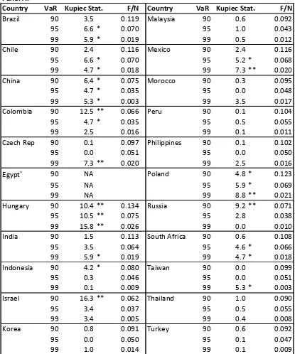
[Insert Table 2]

Table 2, Panel A reports the performance of the VaR for developing countries. The null

hypothesis was rejected at all significance levels for Hungary. There are slightly poor

8

performances of VaR for Colombia, Israel, Mexico, Poland and Russia. Several developing

countries including Korea, Malaysia, Morocco, Peru, Philippines, Thailand and Turkey have

no rejections. It is possible to say that VaR has some value as measure of risk for Indonesia

and for emerging market giants China, Brazil, and India. Table 2, Panel B reports the number

of rejections and non-rejections for Kupiec test. Number of non-rejections is much larger than

the number of rejections. A comparison of Panels B in Tables 1 and 2 clearly reveals that there

was decoupling between emerging and developed countries in terms of market risk during the

global financial crisis.

The two shortcomings of the Kupiec Test are that it does not take into account of the

sequences of violations and it has limited power. To improve on the first shortcoming,

Christoffersen et. al. (2001) design a test which gives emphasis to the predecessor of a

violation. In case the violations are independent, the ratio of preceding violations and

non-violations should not be significantly different.

If we define n_ij as the number of observations i followed by j (i, j=0,1) where 1 indicates

a violation and 0 indicates a non-violation, then the test statistic

        − − − = ₋ F F N n n n n C α α π π π π ) 1 ( ) 1 ( ) 1 ( ln 2 11 10 01 00 11 11 01 01 where

∑

π , follows the χ2 distribution with 2 degrees of freedom. If there is

independence of the violations, then the numerator and denominator will be approximately

same and the test statistic will be close to 0.

9

Table 3 reports the results from the Christoffersen Test for all countries. Note that the test

rejects the appropriateness of VaR for Canada, Denmark, France, Greece, Italy, Netherlands,

Norway, Spain, Sweden, Switzerland, and UK at all levels of significance. Developing

countries for which VaR performs poorly seem to be Colombia, Czech Republic, Hungary,

India, Mexico, Morocco and Poland. The only country with non-rejections at all confidence

levels is Turkey. Table 3, Panel B tabulates the number of rejections and non-rejections for the

developed and developing countries separately. Overall conclusion from Table 3 is that the

developing countries still have less rejections than the developed ones, but the difference is

somewhat smaller when compared to the Kupiec test results reported Table 2 .

The last comparison we make is based on the Quadratic Loss (QL) function. Tests based on

the number of rejections at different confidence levels give an idea about the performance of

VaR as a measure of risk, but they do not take the magnitude of performance loss into

account. Therefore, we make use of a loss function in order to assess the magnitude of the

poor performance of the VaR. Define the QL (Quadratic Loss) function as:

(

)

1

0

t t t t

t

r VaR if r VaR

QL

otherwise

 _{+ − <}



= 

for tth day’s VaR. Since there were no convergences for some cases, we calculate the Average Quadratic Loss (AQL) for each country and for each VaR confidence level to make

comparisons.

[Insert Table 4]

Next we rank countries based on these averages. Table 4, Panel A shows these ranks in

parentheses just below the country names. Among the developed countries, Hong Kong has

10

highest average loss belongs to the securities markets of Norway, Canada and Italy. USA,

Japan and Germany have relatively low AQLs.

Regarding the developing countries, the minimum AQLs belong to Israel and China followed

by Colombia and Russia. The worst performing securities markets in terms of VaR as a

measure of risk are Hungary, Poland, and Brazil. The VaR performs well for Russia and China

but it performs poorly for Brazil and India.

Table 4 Panel B, reports the mean AQL for developed and developing countries at each VaR

confidence level. The mean figures for developing countries are smaller than the ones for

developed countries, providing some additional evidence for the decoupling discussed above.

4. Conclusion

This study examines the performance of Value-at-Risk (VaR) as a risk measure across a large

sample of developed and emerging countries by utilizing unconditional and conditional tests

of Kupiec and Christoffersen, respectively, and the Quadratic Loss Function. There are three

main conclusions from our study. First, the performance of VaR as a risk measure was worse

for developed countries than the developing ones during the global financial crisis. One

possible reason might be that the developed countries have been affected from the crisis more

adversely when compared to the emerging countries. Second, our results reveal some

evidence of decoupling between emerging and developed countries in terms of market risk

during the global financial crisis. Finally, as the rejection of the appropriateness of VaR for

many countries indicates, alternative measures of risk should be used together with VaR and

the performance of these risk measures should be regularly evaluated to improve the

11

continue to hold when other measures of risk together with different methodological choices

12

References

Akın, Ç., and M.A. Kose. 2008. "Changing nature of North–South linkages: Stylized facts and explanations." Journal of Asian Economics 19, no. 1: 1-28.

Ane, T. (2006) " An analysis of the Flexibility of Asymmetric Power GARCH models" Computational Statistics and Data Analysis 51: 931-55.

Angelidis, T, Benos, A. , Degiannakis, S. (2004) "The Use of GARCH Models in VaR Estimation" Statistical Methodology 1: 105-128.

Basel Committee on Banking Supervision, 1994. Risk Management Guidelines for Derivates. Bank for International Settlements, Basel.

Basel Committee on Banking Supervision, 1996. Supplement to the Capital Accord to Incorporate Market Risks. Bank for International Settlements, Basel.

Berkowitz, J., and J. O'Brien. (2002). “How Accurate Are Value-at-Risk Models at Commercial Banks?” Journal of Finance 57, 1093-1111.

Bollerslev, T. (1986) "Generalized Autoregressive Conditional Heteroskedasticity." Journal of Econometrics 31: 307-27

Bollerslev, T. (2008) Glossary to Arch (Garch). CREATES Research Paper 2008-49.

Cannata, Francesco and Quagliariello, Mario, The Role of Basel II in the Subprime Financial Crisis: Guilty or Not Guilty? (January 14, 2009). CAREFIN Research Paper No. 3/09. Available at SSRN: http://ssrn.com/abstract=1330417

Chan, N.H., Deng, S-J., Peng, L. and Xia, Z., 2007. “Interval estimation of value-at-risk based on GARCH models with heavy-tailed innovations.” Journal of Econometrics 137, 556–576.

Christoffersen, P., Hahn, J., Inoue, A., 2001. “Testing and comparing Value-at-Risk measures.” Journal of Empirical Finance 8, 325–342.

Clark, E., Kassimitis, K., 2004. “Country financial risk and stock market performance: the case of Latin America.” Journal of Economics and Business 56 (2004) 21–41.

Dooley, M., and M. Hutchison. 2009. "Transmission of the U.S. subprime crisis to emerging markets: Evidence on the decoupling–recoupling hypothesis." Journal of International Money and Finance 28, no. 8: 1331-1349.

Escanciano, J.C., and Olmo, J. (2011) " Robust Backtesting Tests for Value-at-risk Models."

Journal of Financial Econometrics, 9, No. 1, 132–161.

European Commission, (2009). Economic crisis in Europe: causes, consequences and responses, Office for Official Publications of the European Communities.

13

Fan, Y., Zhang, Y-J. , Trai, H-T., and Wei, Y-M. (2008) " Estimating ‘Value at Risk’ of Crude Oil Price and its Spillover Effect Using the GED-GARCH approach." Energy Economics 30: 3156-3171.

Felices, G., and T. Wieladek. 2012. "Are Emerging Market Indicators of Vulnerability to Financial Crises Decoupling from Global Factors?" Journal of Banking and Finance 36, no. 2: 321-331.

Fidrmuc, J., and I. Korhonen. 2010. "The Impact of the Global Financial Crisis on Business Cycles in Asian Emerging Economies." Journal of Asian Economics 21, no. 3: 293-303.

Frank, N., and H. Hesse. 2009. "Financial Spillovers to Emerging Markets during the Global Financial Crisis." Finance a Uver/Czech Journal of Economics and Finance 59, no. 6: 507-521.

Giot, P. and Laurent, S. (2003) “Market risk in commodity markets: a VaR approach.” Energy Economics, 25, 435–457.

Giot, P. and Laurent, S. (2004) “Modelling Daily Value-at-Risk Using Realized Volatility and ARCH Type Models.” Journal of Empirical Finance, 11: 379-398.

Goodhart, C. A. E. (2008). "The Regulatory Response to the Financial Crisis." Journal of Financial Stability 4(4): 351-358.

Gnamassou, Y.T. (2010) “Value-at-risk prediction: a comparison of alternative techniques applied to a large sample of individual stock data.”, MS thesis, HEC Montreal.

Hartz, C. Mittnik, S. & Paolella, M. (2006) " Accurate Value-at-Risk Forecasting Based on the Normal-GARCH Model." Computational Statistics and Data Analysis 51: 2295-2312.

Kim, S.; J.-W. Lee; and C.-Y. Park. 2011. "Emerging Asia: Decoupling or Recoupling." World Economy 34, no. 1: 23-53.

Kose, M.A.; C. Otrok; and E.S. Prasad. 2008. "Global Business Cycles: Convergence or Decoupling?" National Bureau of Economic Research Working Paper Series No. 14292

Kupiec, P.H., 1995. “Techniques for verifying the accuracy of risk measurement models.” Journal of Derivatives 3, 73–84.

McAleer, M., Veiga, B., and Hoti, S. (2011) “Value-at-Risk for country risk ratings”, Mathematics and Computers in Simulation, 81, 1454–1463

Poon, S.-H. & Granger, C. W. J. (2003) "Forecasting Volatility in Financial Markets: A Review." Journal of Economic Literature 41: 478-539.

Orhan, M. and Köksal, B., 2012 “A Comparison of GARCH Models for VaR Estimation”, Expert Systems with Applications, 39, 3582-2592, 2012.

14

So, M.K.P. and Yu, P.L.H., 2006 “Empirical analysis of GARCH models in value at risk estimation”, Int. Fin. Markets, Inst. and Money 16 180–197.

Tang, T-L, Shieh, S-J. (2006) “Long Memory in Stock Index Futures Markets: A Value-At-Risk Approach”, Physica A, 306, 437-448.

Tett, G. “Genesis of the debt disaster”, Financial Times, May 1, 2009.

Uckun, D., and M. Doerr. 2010. "Emerging Markets: Theory and Practice/Turkey's Reforms Post 2001 Crisis." Journal of Global Analysis 1, no. 1: 51-73.

15

0

5

0

0

0

1

0

0

0

0

1

5

0

0

0

01.01.07 01.01.08 01.01.09 01.01.10 01.01.11 01.01.12

Developed Countries

Developed countries excluding Greece, Spain, and Portugal

Emerging Countries

Source. Bloomberg

Note. CDS Index=100 for 01/01/2007 for each country. The rest of the index is calculated based on percentage changes in CDS spreads. Then average index is calculated for developed and developing countries that have data starting from January 2007.

Developed Countries:Austria, Belgium, France, Germany, Greece, Italy, Japan, Portugal, Spain, Sweden. Emerging Countries: Brazil, Chile, China, Colombia, Czech Rep., Hungary, Indonesia, Israel, S. Korea, Malaysia, Mexico, Peru, Philippines, Poland, Russia, S. Africa, Thailand, Turkey.

16

Panel A.

Country VaR F/N Country VaR F/N

Australia 90 2.4 0.116 Italy 90 11.8 ** 0.136 95 12.4 ** 0.078 95 15.3 ** 0.081 99 26.5 ** 0.032 99 15.8 ** 0.026 Austria 90 12.5 ** 0.137 Japan 90 1.8 0.114 95 23.3 ** 0.089 95 4.0 * 0.065 99 12.1 ** 0.024 99 1.7 0.015 Belgium 90 7.4 ** 0.128 Netherlands 90 1.0 0.110 95 23.3 ** 0.089 95 6.6 * 0.070 99 12.1 ** 0.024 99 7.3 ** 0.020 Canada 90 15.5 ** 0.142 Norway 90 24.4 ** 0.153 95 27.1 ** 0.092 95 29.8 ** 0.095 99 44.6 ** 0.039 99 31.3 ** 0.034 Denmark 90 3.1 0.118 Portugal 90 0.0 0.101 95 4.0 * 0.065 95 1.3 0.059 99 10.4 ** 0.023 99 1.7 0.015 Finland 90 0.0 0.100 Singapore 90 0.8 0.109 95 2.5 0.062 95 0.5 0.055 99 0.1 0.011 99 4.7 * 0.018 France 90 7.4 ** 0.128 Spain 90 9.1 ** 0.132 95 9.7 ** 0.074 95 7.3 ** 0.071 99 10.4 ** 0.023 99 10.4 ** 0.023 Germany 90 0.5 0.107 Sweden 90 10.4 ** 0.134 95 3.5 0.064 95 9.7 ** 0.074 99 5.9 * 0.019 99 8.8 ** 0.021 Greece 90 4.8 * 0.123 Switzerland 90 4.8 * 0.123 95 12.4 ** 0.078 95 8.9 ** 0.073 99 13.9 ** 0.025 99 19.8 ** 0.028 Hongkong 90 4.2 * 0.080 UK 90 5.8 0.125 95 3.4 0.037 95 12.4 ** 0.078 99 5.3 * 0.003 99 17.7 ** 0.027 Ireland 90 6.3 * 0.126 USA 90 0.5 0.107 95 15.3 ** 0.081 95 2.5 0.062 99 5.9 * 0.019 99 5.9 * 0.019

Table 1. Kupiec Test Results, Developed Countries.

**, and * denote rejections at the 1%, and 5% levels, respectively. F/N is the proportion of

violations. The critical values for 1%, and 5% significance levels of the Chi-Square

Distribution with 1 degree of freedom are 6.64, and 3.84, respectively.

Kupiec Stat. Kupiec Stat.

Panel B.

# of non-rejections VaR 1% Level 5% Level

90 8 12 10

95 13 16 6

99 14 19 3

Total 35 47 19

17

Panel A.

Country VaR F/N Country VaR F/N

Brazil 90 3.5 0.119 Malaysia 90 0.6 0.092 95 6.6 * 0.070 95 1.0 0.043 99 5.9 * 0.019 99 0.5 0.012 Chile 90 2.4 0.116 Mexico 90 2.4 0.116 95 6.6 * 0.070 95 5.2 * 0.068 99 4.7 * 0.018 99 7.3 ** 0.020 China 90 6.4 * 0.075 Morocco 90 0.3 0.095 95 4.7 * 0.035 95 0.0 0.048 99 5.3 * 0.003 99 3.5 0.017 Colombia 90 12.5 ** 0.066 Peru 90 0.1 0.104 95 4.7 * 0.035 95 0.5 0.055 99 2.5 0.016 99 0.1 0.011 Czech Rep 90 0.1 0.097 Philippines 90 0.1 0.102 95 0.0 0.051 95 0.0 0.050 99 7.3 ** 0.020 99 2.5 0.016 Egypt+ 90 NA Poland 90 4.8 * 0.123

95 NA 95 5.9 * 0.069

99 NA 99 8.8 ** 0.021

Hungary 90 10.4 ** 0.134 Russia 90 9.2 ** 0.071 95 10.5 ** 0.075 95 2.8 0.038 99 15.8 ** 0.026 99 0.0 0.010 India 90 1.5 0.113 South Africa 90 0.6 0.108 95 3.5 0.064 95 4.6 * 0.066 99 5.9 * 0.019 99 4.7 * 0.018 Indonesia 90 4.2 * 0.080 Taiwan 90 0.0 0.099 95 0.3 0.046 95 0.0 0.051 99 0.1 0.009 99 5.3 * 0.003 Israel 90 16.3 ** 0.062 Thailand 90 1.0 0.090 95 3.4 0.037 95 0.5 0.055 99 3.4 0.005 99 0.4 0.008 Korea 90 0.8 0.091 Turkey 90 0.6 0.092 95 0.0 0.050 95 0.1 0.047 99 1.0 0.014 99 0.1 0.009

+ : Insufficient number of convergences for Egypt.

**, and * denote rejections at the 1%, and 5% levels, respectively. F/N is the proportion of violations. The critical values for 1%, and 5% significance levels of the Chi-Square Distribution with 1 degree of freedom are 6.64, and 3.84, respectively.

Table 2. Kupiec Test Results, Developing Countries.

18

Panel B.

# of non-rejections VaR 1% Level 5% Level

90 4 7 14

95 1 8 13

99 4 10 11

Total 9 25 38

19

VaR Country Country Country Country

90 Australia 4.28 Italy 24.86 ** Brazil 9.96 ** Malaysia 6.32 *

95 18.12 ** 18.48 ** 13.30 ** 12.49 **

99 27.68 ** 30.15 ** 8.20 * 2.90

90 Austria 30.67 ** Japan 2.27 Chile 17.61 ** Mexico 11.84 **

95 44.53 ** 5.43 18.04 ** 24.04 **

99 12.54 4.24 6.99 * 11.18 **

90 Belgium 25.29 Netherlands 22.41 ** China 13.02 ** Morocco 29.06 **

95 41.70 20.79 ** 5.49 19.04 **

99 23.09 ** 20.84 ** 10.69 ** 20.24 **

90 Canada 27.26 ** Norway 33.61 ** Colombia 28.86 ** Peru 14.09 **

95 28.99 ** 38.13 ** 17.26 ** 8.65 *

99 51.09 ** 37.04 ** 13.87 ** 3.08

90 Denmark 23.62 ** Portugal 7.29 * Czech R. 13.50 ** Philippines 8.59 *

95 18.09 ** 1.73 10.39 ** 3.16

99 13.54 ** 4.24 15.54 ** 4.12

90 Finland 11.55 ** Singapore 5.33 Egypt+ NA Poland 20.04 **

95 7.94 * 2.39 NA 23.88 **

99 3.08 5.82 NA 9.48 **

90 France 17.65 ** Spain 15.08 ** Hungary 28.80 ** Russia 22.71 **

95 14.79 ** 11.72 ** 24.13 ** 17.15 **

99 13.54 ** 13.54 ** 21.25 ** 3.12

90 Germany 8.79 * Sweden 18.18 ** India 16.64 ** S. Africa 3.19

95 6.43 * 13.15 ** 12.63 ** 5.85

99 6.90 * 11.01 ** 10.22 ** 9.41 **

90 Greece 12.85 ** Switzerland 14.45 ** Indonesia 23.35 ** Taiwan 0.23

95 20.06 ** 23.82 ** 13.27 ** 1.31

99 19.83 ** 21.59 ** 3.74 10.69 **

90 Hong Kong 11.01 ** UK 11.53 ** Israel 16.55 ** Thailand 11.42 **

95 7.86 * 16.43 ** 5.47 14.65 **

99 10.69 ** 19.76 ** 10.01 ** 4.62

90 Ireland 14.41 ** USA 0.78 Korea 4.00 Turkey 3.53

95 23.65 ** 3.36 5.34 3.91

99 6.90 * 8.20 * 8.00 * 3.42

Table 3. Christoffersen Test Results

Developed Countries Developing Countries

+ : Insufficient number of convergences for Egypt.

Chris.Test Chris.Test Chris.Test Chris.Test

20

Panel B.

# of non-rejections

# of non-rejections VaR 1% Level 5% Level 1% Level 5% Level

90 15 17 5 15 17 4

95 14 17 5 13 14 7

99 14 17 5 11 14 7

Total 43 51 15 39 45 18

# of rejections

Developed Countries Developing Countries

21

Panel A.

VaR Country AQL Country AQL Country AQL Country AQL

90 Australia 0.116 Italy 0.136 Brazil 0.119 Malaysia 0.092

95 (12) 0.078 (19) 0.081 (16) 0.070 (6) 0.043

99 0.032 0.026 0.019 0.012

90 Austria 0.137 Japan 0.114 Chile 0.116 Mexico 0.116

95 (20) 0.089 (7) 0.065 (15) 0.070 (15) 0.068

99 0.024 0.015 0.018 0.020

90 Belgium 0.128 Netherlands 0.110 China 0.075 Morocco 0.095

95 (18) 0.089 (8) 0.070 (2) 0.035 (10) 0.048

99 0.024 0.020 0.003 0.017

90 Canada 0.142 Norway 0.153 Colombia 0.066 Peru 0.104

95 (20) 0.092 (21) 0.095 (3) 0.035 (12) 0.055

99 0.039 0.034 0.016 0.011

90 Denmark 0.118 Portugal 0.101 Czech R. 0.097 Philippines 0.102

95 (9) 0.065 (3) 0.059 (11) 0.051 (11) 0.050

99 0.023 0.015 0.020 0.016

90 Finland 0.100 Singapore 0.109 Egypt NA Poland 0.123

95 (2) 0.062 (4) 0.055 NA (17) 0.069

99 0.011 0.018 NA 0.021

90 France 0.128 Spain 0.132 Hungary 0.134 Russia 0.071

95 (11) 0.074 (15) 0.071 (18) 0.075 (4) 0.038

99 0.023 0.023 0.026 0.010

90 Germany 0.107 Sweden 0.134 India 0.113 S. Africa 0.108

95 (6) 0.064 (16) 0.074 (14) 0.064 (13) 0.066

99 0.019 0.021 0.019 0.018

90 Greece 0.123 Switzerland 0.123 Indonesia 0.080 Taiwan 0.099

95 (13) 0.078 (10) 0.073 (5) 0.046 (8) 0.051

99 0.025 0.028 0.009 0.003

90 Hong Kong 0.080 UK 0.125 Israel 0.062 Thailand 0.090

95 (1) 0.037 (17) 0.078 (1) 0.037 (8) 0.055

99 0.003 0.027 0.005 0.008

90 Ireland 0.126 USA 0.107 Korea 0.091 Turkey 0.092

95 (14) 0.081 (5) 0.062 (9) 0.050 (7) 0.047

99 0.019 0.019 0.014 0.009

Developed Countries Developing Countries

Table 4. Average Quadratic Loss

Panel B.

VaR Developed Countries Developing Countries

90 0.121 0.097

95 0.072 0.053