http://www.scirp.org/journal/ojmh ISSN Online: 2163-0496 ISSN Print: 2163-0461
Application of the Reciprocal Analysis for Sensible
and Latent Heat Fluxes with Evapotranspiration at
a Humid Region
Toshisuke Maruyama
*, Manabu Segawa
Faculty of Environmental Science, Ishikawa Prefectural University, Ishikawa, Japan
Abstract
Evapotranspiration acts an important role in hydrologic cycle and water resources planning. But the estimation issue still remains until nowadays. This research at-tempts to make clear this problem by the following way. In a humid region, by ap-plying the Bowen ratio concept and optimum procedure on the soil surface, sensible and latent heat fluxes are estimated using net radiation (Rn) and heat flux into the ground (G). The method uses air temperature and humidity at a single height by re-ciprocally determining the soil surface temperature (Ts) and the relative humidity (rehs). This feature can be remarkably extended to the utilization. The validity of the method is confirmed by comparing of observed and estimated latent (lE) and sensi-ble heat flux (H) using the eddy covariance method. The hourly change of the lE, H, Ts and rehs on the soil surface, yearly change of lE and H and relationship of esti-mated lE and H versus observed are clarified. Furthermore, monthly evapotranspira-tion is estimated from the lE. The research was conducted using hourly data of FLUXNET at a site of Japan, three sites of the United States and two sites of Europe in humid regions having over 1000 mm of annual precipitation.
Keywords
Bowen Ratio, Eddy Covariance, Reciprocal Determination, Estimation of Sensible and Latent Heat Fluxes, Soil Surface Temperature and Humidity
1. Introduction
In the natural world, the air temperature and humidity are determined by H and lE from the net radiation (Rn) and heat flux into the ground (G). Therefore, our research attempts the reciprocal analysis of H and lE from the air temperature (Tz) and humidity How to cite this paper: Maruyama, T. and
Segawa, M. (2016) Application of the Reci-procal Analysis for Sensible and Latent Heat Fluxes with Evapotranspiration at a Humid Region. Open Journal of Modern Hydrolo-gy, 6, 230-252.
http://dx.doi.org/10.4236/ojmh.2016.64019
Received: August 17, 2016 Accepted: October 17, 2016 Published: October 20, 2016
Copyright © 2016 by authors and Scientific Research Publishing Inc. This work is licensed under the Creative Commons Attribution International License (CC BY 4.0).
http://creativecommons.org/licenses/by/4.0/
(rehz) at single height while satisfying the heat balance relationship. The concept can’t find the other relevant methods, and it only requires Rn, G, Tz and rehz. This feature is remarkably widened a utilization purposes.
Recently, we reported the reciprocal analysis of sensible and latent heat fluxes in a forest region [1]. However, “humid region” is quite different from “forest region” be-cause of no canopy. This paper described “humid region” instead of “forest region”, al-though there was similar concept in previous research.
The main different point is: the present paper contains two unknown variables, i.e., relative humidity (rehs) and temperature on the soil surface (Ts) while the previous paper contains only one variable, i.e., rehs, on the canopy surface. Therefore, the analy-sis has differences in that the present paper has to solve two simultaneous equations while the previous paper solved only one equation. In the analytical process, various new points arisen. Addition, this paper describes the comparison of the Penman me-thod with our meme-thod because of humid region.
In the proposed method, the unknown variables, Ts and rehs were determined by the non-linear optimization technique known as the general reduced gradient (GRG) using the Excel Solver (Appendix 1).
2. Materials
We proposed a general method for estimating sensible and latent heat flux using single height temperature and humidity. The method contains two unknown variables: soil surface temperature, Ts, and humidity, rehs. This chapter describes the theoretical back- ground for estimating Ts and rehs, the practical procedure, data correction, the details of test sites and measurement instruments.
2.1. Method of Analysis
2.1.1. Fundamental Concept of the Model
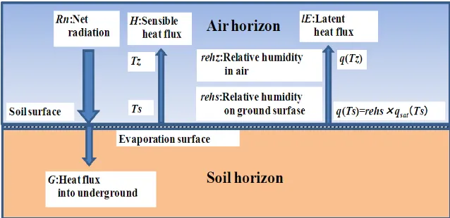
[image:2.595.213.532.534.689.2]A proposed model is somewhat similar to previous research [1]. Therefore, briefly the outline is described. The proposed model considers the near-soil surface as shown in
Figure 1.
Here, Rn is net radiation which is portioned into sensible, latent and underground heat fluxes. Ts is the soil surface temperature, Tz is the air temperature at height z,
( )
q Tz is the specific moisture at height z, rehz is relative humidity in air at height z,
( )
q Ts is the unsaturated specific moisture on the soil surface, and qsat
( )
Ts is thesaturated specific moisture on the soil surface.
The fundamental formulae of the model satisfy the following well-known heat bal-ance relationship [2].
Rn=H+lE+G. (1)
Here, Rn is the net radiation flux (W∙m−2), G is the heat flux into the ground (W∙m−2),
H is the sensible heat flux (W∙m−2), and lE is the latent heat flux (W∙m−2).
In addition, the Bowen ratio (H/lE) is defined as follows [2]:
(
)
(
1 2)
01 2
Cp T T
B
l q q
− =
− . (2)
We apply the concept of Bowen ratio to the layer between the soil surface and obser-vation height of Tz and rehz. But, the Ts and q Ts
( )
are just on the surface and usuallyunknown.
2.1.2. Governing Equation for Estimating the Unknown Variables Ts and rehs The governing equation to be solved is obtained by heat balance relationship [1]. The unknown variables Ts and rehs are estimated as follows: The Ts and the q Ts
( )
, i.e.,rehs × esat(Ts) are assumed initially; thus, the heat balance relationship has not closed
as Equation (3):
, , 1, 2, 3,
n est i eat i i
R − −G H −lE =ε i= ⋅⋅⋅n (3)
(
)
(
)
( )
, ,
,
, ,
s ass z
est i app i
est i s ass z
Cp T T
H B
lE l q T q T
−
= =
−
(4)
, 1
, 1
est i
app i Rn G lE
B
+
− =
+ and Hest i,+1=Bapp i, ×lEest i,+1. (5)
Here i is number of iteration. Hest,i is estimated sensible heat flux in i times iteration,
lEest,i is estimated latent heat flux, εi is residual of heat balance relationship of i times
iteration, Tsassis assumed soil surface temperature, q Ts
(
ass)
is specific moisture atTsass, Bapp is apparent ratio of sensible and latent heat flux under convergence process.
The approximated Ts and rehs putting in Equation (4), lE and H of next order ap-proximated values obtained by Equation (5).
By repeating the above calculation from Equation (3) to Equation (5), the Bapp
con-verged to B0 according to objective function ABS (εi) conversed to a minimum.
After optimization, Bappisconversed to B0. Then, lEest and Hest can be obtained as
fol-lows:
0 1
est
Rn G lE
B
− =
+ and Hest =B0×lEest. (6)
0
s To
T = ×G D Kt RTs T× + . (7)
Here, T0 is the observed soil temperature (˚C), DTois the depth of the temperature
observation (cm), Kt is the assumed thermal conductivity (W∙m−1∙˚C−1).
Equation (7) describes how to obtained Ts by extrapolating T0 using G, DTo and Kt.
The calculation follows General Reduced Gradient (GRG) algorithm, which can be ap-plied with the Excel Solver on a personal computer (Appendix 1 and Appendix 2).
2.1.3. General Solution
To uniquely determine the two unknown variable Ts and rehs, two equations are re-quired mathematically. We set the two equations as follows assuming Ts and rehs has no remarkable difference between two unit hours:
, ,
j j j j j
n est i est i i
R −G −H −lE =
ε
(8)1 1 1 1 1
, ,
j j j j j
n est i est i i
R + −G + −H + −lE + =
ε
+ . (9)Here, j is the order of hours from 1 to the end of the analyzed hours and i is the number of iterations.
The calculation is performed by solving Equation (8) and Equation (9) simulta-neously under Tj= Tsj+1 and rehj= rehsj+1conditions: 1
ABS j ABS j
i i
ε= ε + ε +
con-versed to minimum.
In addition, to prevent abnormal fluctuation of Hest versus lEest in optimization process,
constraints Rn − G < H, lE are applied as follows (Equation (10)):
( )
(
)
{
}
{
(
)
(
)
}
( )
(
)
{
}
{
(
)
(
)
}
1 1 1
1 1 1
ABS ABS ABS ABS for
ABS ABS ABS ABS for
j j j j j j
j j j j j j
H H Rn G Rn G H
lE lE Rn G Rn G lE
+ + +
+ + +
+ < − + −
+ < − + − . (10)
Equation (8) and Equation (9) are nonlinear two element simultaneous equations. The two unknown variables can be estimated for the limit to which ε is minimized, al-lowing H and lE to be estimated. Note that the other factors were obtained from obser-vations or were calculated independently.
2.1.4. Correction of the Heat Imbalance Based on Multiple Regression Analysis
The heat imbalance is observed in actual data, which is well known as a “closure issue”
[3][4]. Therefore, the data was corrected conventionally according to Allen’s procedure by multiple regression analysis [5]:
Rn− = ×G A lE+ ×B H. (11)
Here: Rn, G, lE and H are described earlier. A, B are the regression coefficient for lE, H.
To guarantee the heat balance relationship, all sites used the corrected data. In addi-tion, the correction is conducted using the daily basis.
2.1.5. Constraint to Improve the Underestimation of lE
( ) ( ) ( )
q Ts q Tzb q Ts Ts
Ts Tz
−
= − ×
− (12)
b is a constant passing through straight line at T = 0˚C with slope
( ) ( ) (
)
q Ts −q Tz Ts Tz−
. In Equation (12) the q Ts
( )
and q Tz( )
are converted from( )
e Ts and e Tz
( )
using q Ts( )
and e Ts( )
relationship.The constraint for optimization process set as follows:
0
b≤ or b≥0. (13)
The constraint is expected increasing of lEest, whereas decrease Hest at high humidity
area or vice versa. General analysis applied the constraint of Equation (13).
In addition, the constraints of Equation (13) have a similar role of rehs > rehz or rehs < rehz depending on initial values of rehs = rehz or rehs = 1.0 that is expected in humid region.
2.1.6. Initial Values forOptimization and Constraints
The initial values of Ts and rehs are key factors for obtaining reliable results. The value of Ts is chosen as T0 because the T0 is observed at near the soil surface. The initial value
of rehs chosen as rehs = 1.0 because humid region or rehs = rehz depending on site specific conditions. Then, RTs was assumed to be 0, The RTs was automatically im-proved to satisfy the optimum value of Ts and rehs.
The ε has very small values on the order of 10−15 W∙m−2 initially, because B
app nearly
satisfies the heat balance relationship. Therefore, the objective function is multiplied by 1015. To avoid abnormal fluctuation of H and lE, in the optimization process,
con-straints on those are set as less than (Rn − G) as mentioned earlier. Additionally, Bapp is
constrained as −100 < Bapp < 100 by referring to the actual data and optimization process
[1]. The reason is described in the discussion section. We set the precision: =0.000001 and convergence: =0.0001 in Solver option.
2.2. Investigation Sites and Equipment
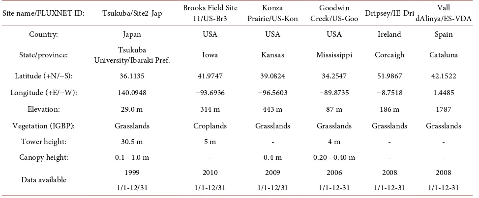
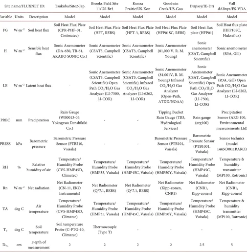
To examine the proposed method, six sites were chosen in humid regions having an-nual precipitation over 1000 mm (Table 1), including a site in Japan, three sites in the USA and two sites in Europe. Site2-Jap data in Japan were prepared by Tukuba Univer-sity (2006) [6]. Three sites in USA data were prepared by AmeriFlux (Brooks Field Site 11 of US-Br3 [7], Konza Prairie of US-Kon [8], Goodwin Creek of US-Goo [9]). And two sites of Europe data prepared by European Fluxes Database Cluster (Vall dAlinya of ES-VDA [10] and Dripsey of IE-Dri] [11].
H was observed by eddy covariance at all sites (Hobs). lE was also observed by eddy
covariance at five sites (lEobs) excluding site2-Jap. The lEobs at site2-Jap was estimated by
imbalance (lEimb= Rn – G − Hobs). Rn and G were observed at all sites. As shown in
Ta-ble 2, the soil temperature T0 was observed by thermometer at the depth of 2 ~ 5 cm.
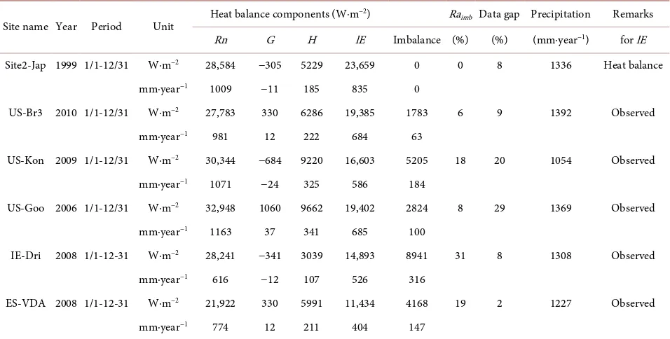
2.3. Heat Balance Relationship of Observed Sites and Data Gap
ex-pressed in heat flux. The imbalance was observed at USA and European sites because directory observed lE by the eddy covariance. US-Kon, IE-Dri and ES-VPA has re-markable large imbalance of 18%, 31% and 19%. The imbalance is zero at the site2-Jap because no observed of lE.
Site2-Jap, US-Br3, IE-Dri and ES-VPA have relatively small data gap while US-Kon and US-Goo have remarkable. The time of having data gap is avoided in the analysis. The annual precipitation of the examined year is shown.
3. Result
The general solution determines two variables, Ts and rehs, using two equations simul-taneously. Therefore, Ts and rehs can be uniquely determined mathematically. The ini-tial value is set as aforementioned. Furthermore, the heat balance is not achieved in-stantaneously; it requires a few hours [5]. Thus, the hourly figure adjusts to a five-hour moving average.
3.1. Conversion of Observed Data (
H
obsand
lE
obs) into Corrected Data
(
H
corand
lE
cor)
Observed data do not achieve the heat balance relationship, as shown in Table 3. To maintain the relationship, multiple regression analysis is applied using Equation (11).
Figure 2 describes the relationship (Rn − G) versus (H + lE) of the original and cor-rected data in which the observed data are shown in the red circle while the corcor-rected data are shown in the blue circle. The slope of the five tested sites increased and ap-proached to 1.0. The regression coefficients described in Table 4 are A for H and B for lE. The observed data are corrected by these coefficients for all of the tested sites.
3.2. Comparison of the Hourly Change of the
lE
and
H
at all Sites
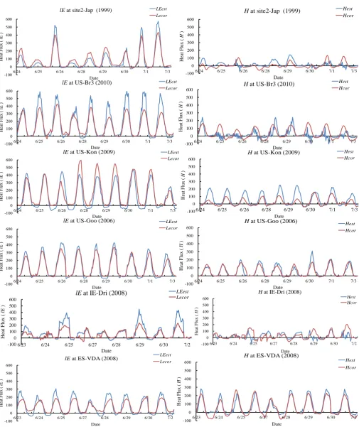
[image:6.595.72.559.506.708.2]To confirm the validity, Figure 3 compares the hourly changes in lEobs with lEest and
Table 1. Features of the tested sites.
Site name/FLUXNET ID: Tsukuba/Site2-Jap Brooks Field Site 11/US-Br3 Prairie/US-Kon Konza Creek/US-Goo Dripsey/IE-Dri Goodwin dAlinya/ES-VDA Vall
Country: Japan USA USA USA Ireland Spain
State/province: University/Ibaraki Pref. Tsukuba Iowa Kansas Mississippi Corcaigh Cataluna
Latitude (+N/−S): 36.1135 41.9747 39.0824 34.2547 51.9867 42.1522
Longitude (+E/−W): 140.0948 −93.6936 −96.5603 −89.8735 −8.7518 1.4485
Elevation: 29.0 m 314 m 443 m 87 m 186 m 1787
Vegetation (IGBP): Grasslands Croplands Grasslands Grasslands Grasslands Grasslands
Tower height: 30.5 m 5 m - 4 m - -
Canopy height: 0.1 - 1.0 m - 0.4 m 0.20 - 0.40 m - -
Data available 1999 2010 2009 2006 2008 2008
Table 2. Measurement instruments of the tested sites including DTo.
Site name/FLUXNET ID: Tsukuba/Site2-Jap Brooks Field Site 11/US-Br3 Prairie/US-Kon Konza Creek/US-Goo Goodwin Dripsey/IE-Dri dAlinya/ES-VDA Vall
Variable Units Description Model Model Model Model Model Model
FG W∙m−2 Soil heat flux Soil Heat Flux Plate (CPR-PHF-01,
Cmimatec)
Soil Heat Flux Plate
(HFT, REBS) Soil Heat Flux Plate (HFT-3, REBS) Soil Heat Flux Plate (HFP01SC, REBS) plate (HFP01) Soil Heat flux
Soil Heat flux plate (HFP10SC, Hukseflux)
H W∙m−2 Sensible heat
flux
Sonic Anemometer (DA-650, TR-61, AKAIJO SONIC Co.)
Sonic Anemometer (CSAT3, Campbell Scientific) Sonic Anemometer (CSAT3, Campbell Scientific) Sonic Anemometer (81,000 V, R. M.
Young) Sonic anemometer (CSAT, Campbell Scientific) Sonic anemometer (R3A, Gill)
LE W∙m−2 Latent heat flux -
Sonic Anemometer (CSAT3, Campbell Scientific) Open Path CO2/H2O Gas
Analyzer (LI-7500, LI-COR)
Sonic Anemometer (CSAT3, Campbell Scientific) Infrared CO2/H2O Gas
Analyzer (LI-6262, LI-COR)
Sonic Anemometer (81,001V, R. M. Young) Infrared CO2/H2O Gas
Analyzer (Open-Path, ATDD/NOAA) Sonic Anemometer (CSAT, Campbell Scientific) Open Path CO2/H2O
Gas Analyzer (LI-7500, LI-COR)
Sonic Anemometer (R3A, Gill) Open Path CO2/H2O Gas
Analyzer (LI-6262, LI-COR)
PREC mm Precipitation
Rain Gauge (WB0013-05, Yokogawa Denshikiki Co.) - - Tipping Bucket Rain Gauge (TB3,
Hydrological Services)
Rain gauge (arg100)
Precipitation Sensor (ARG 100,
Environmental measurements Ltd)
PRESS kPa Barometric pressure Barometric Pressure Sensor (PTB210,
Vaisala) - -
Barometric Pressure Sensor (PTB101, Vaisala) Barometric Pressure Sensor (PTB1001, Vaisala) Sensor technics (model 144SC0811BARO)
RH % humidity of air Relative
Temperature/ Humidity Probe (CVS-HMP45D, Climatec) Temperature/ Humidity Probe (HMP35, Vaisala) Temperature/ Humidity Probe (HMP45C, Vaisala) Temperature/ Humidity Probe (HMP50Y, Vaisala) Temperature/ Humidity Probe (HMP45C, Vaisala) Temperature & humidity transmitter (MP100, Rotronic)
Rn W∙m−2 Net radiation Net Radiometer (CN-11, EKO
Instruments)
Net Radiometer
(Q*7.1, REBS) Net Radiometer (Q*7.1, REBS)
Net Radiometer (Kipp-zonen, CNR1) Net Radiometer (CNR1, Kipp-zonen) Net Radiometer (CNR1, Kipp-zonen)
TA deg C temperature Air
Temperature/ Humidity Probe (CVS-HMP45D, Climatec) Temperature/ Humidity Probe (HMP35, Vaisala) Temperature/ Humidity Probe (HMP45C, Vaisala) Temperature/ Humidity Probe (HMP50Y, Vaisala) Temperature/ Humidity Probe (HMP45C, Vaisala) Temperature & humidity transmitter (MP100, Rotronic)
T0 deg C temperature Soil
Soil temperature Probe (C-PTG-10,
Climatec)
Thermocouple
(Type T) - - - -
DTo cm measurement Depth of 2 2 2 2 2.5 5
Data store: every 30 minutes, hourly.
Hobs or Hest at the six sites in summer. All sites data are reproduced well.
However, in detail, lEest is coincided very well with lEcor excluding IE-Dri whereas Hest
also very well coincided with Hcor without US-Kon. The small differences of Hest may
have a little reflected to the lEest. The other terms, such as lEobs and Hobs describe almost
Table 3. Heat balance of the sites including data gap and annual precipitation (unit: heat flux).
Site name Year Period Unit Heat balance components (W∙m
−2) Ra
imb Data gap Precipitation Remarks
Rn G H lE Imbalance (%) (%) (mm∙year−1) for lE
Site2-Jap 1999 1/1-12/31 W∙m−2 28,584 −305 5229 23,659 0 0 8 1336 Heat balance
mm∙year−1 1009 −11 185 835 0
US-Br3 2010 1/1-12/31 W∙m−2 27,783 330 6286 19,385 1783 6 9 1392 Observed
mm∙year−1 981 12 222 684 63
US-Kon 2009 1/1-12/31 W∙m−2 30,344 −684 9220 16,603 5205 18 20 1054 Observed
mm∙year−1 1071 −24 325 586 184
US-Goo 2006 1/1-12/31 W∙m−2 32,948 1060 9662 19,402 2824 8 29 1369 Observed
mm∙year−1 1163 37 341 685 100
IE-Dri 2008 1/1-12-31 W∙m−2 28,241 −341 3039 14,893 8941 31 8 1308 Observed
mm∙year−1 616 −12 107 526 316
ES-VDA 2008 1/1-12-31 W∙m−2 21,922 330 5991 11,434 4168 19 2 1227 Observed
mm∙year−1 774 12 211 404 147
Note: Data gap is not available data for analysis, i.e., lacked one of which G, Tz, T0, P, erhz, Rn, Hobs and lEobs. Imbalance is estimated by Imb = Rn – G – lE −
H using yearly observed data and the imbalance ratio defined as Raimb = Imb/(Rn − G). 100W∙m−2 = 3.53 mm∙day−1 [12].
rehs set as follows: US-Kon and US-Goo are rehs = rehz with constrains b < 0 and the other sites uses rehs = 1.0 with constrains b > 0.
3.3. Annual Change of the Estimated and Observed
lE
and
H
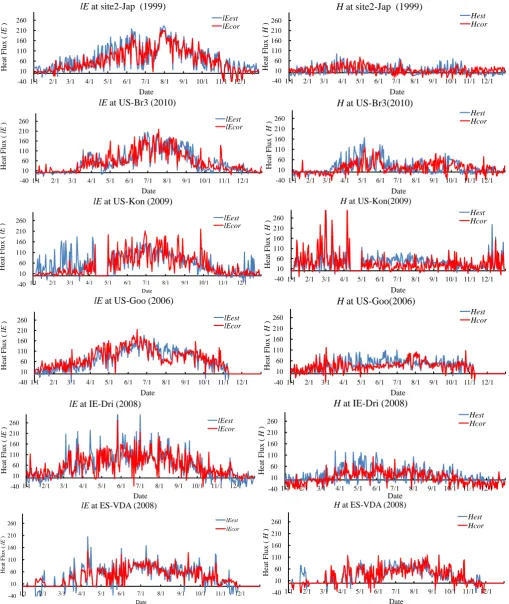
Figure 4 describes the yearly changes of the estimated and observed lE and H for the six sites. All sites describe that the trend relatively well reproduced. However in detail, the results show small differences at spring of lEest at US-Kon. It shows overestimate for
lEest while shows underestimate for Hest. The other terms of lEobs exhibits similar trends
and Hobs also display the same trend but with small differences (not shown).
3.4. Comparison of the Observed and Estimated
lE
and
H
Figure 5 compares the relationship of lE and H on daily basis to confirm the validity of the general solution. If the slope (slope of the straight line) is 1.0, the observed value coincides are well with the estimated values. For lEest, all sites well reproduced (±15%)
whereas lEest are underestimated (>15%) excludes US-Goo. R2 (R is corrected
determi-nation coefficient) of lEest shows underestimated at US-Kon (>60%) and R2 for Hest
show remarkably small values excludes ES-VDA. In addition, the criteria of accuracy (±15%) were determined referring to observed data (Table 3).
3.5. Relationship of the
rehz
and
T
0and Estimated
rehs
and
Ts
Figure 2. Comparison of (Rn − G) with (H + lE) observed and corrected (W∙m−2).
Table 4. Regression coefficient for lE and H.
Site Name A B R2
Site2-Jap 1.000 1.000 0.997
US-Br3 1.164 1.030 0.927
US-Kon 1.186 1.123 0.835
US-Goo 1.082 1.252 0.970
IE-Dri 1.135 1.496 0.916
ES-VDA 1.435 1.472 0.976
Average 1.167 1.229 0.937
A is regression coefficient for lE, B is regression coefficient for H.
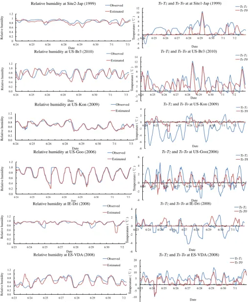
change of rehs and rehz in summer. The figure describes the well functioned optimiza-tion process because the rehs changed remarkably from initial values of 100% of rehz. Difference of rehs and rehz is quite small at all sites. The right hand side of Figure 6
y = 0.9552x R² = 0.8971
y = 0.9178x R² = 0.8966
-100 0 100 200 300
-100 0 100 200 300
H
+
lE
Rn-G
Rn-G
versus
H+lE
at US-Br3
Hcor+lEcor
Hobs+lEobs
y = 0.8426x R² = 0.622
y = 0.7655x R² = 0.6065
-100 0 100 200 300 400
-100 0 100 200 300 400
H
+
lE
Rn-G
Rn-G
versus
H+lE
at US-Kon
Hcor+lEcor
Hobs+lEobs
y = 0.9732x R² = 0.9128
y = 0.8141x R² = 0.9119
-100 0 100 200 300
-100 0 100 200 300
H
+
lE
Rn-G
Rn-G
versus
H+lE
at US-Goo
Hcor+lEcorHobs+lEobs
y = 0.7324x R² = 0.5809
y = 0.6253x R² = 0.5111
-100 0 100 200 300
-100 0 100 200 300
H
+
lE
Rn-G
Rn-G
versus
H+lE
at IE-Dri
Hcor+lEcor
Hobs+lEobs
y = 0.9784x R² = 0.9564
y = 0.6723x R² = 0.9565
-100 0 100 200 300 400 500
-100 0 100 200 300 400 500
H
+
lE
Rn-G
Rn-G
versus
H+lE
at ES-VDA
Figure 3. Hourly changes of lE and H observed and estimated (W∙m−2) (general solution). Note: 1) Initial condition at site2-Jap, US-Br3,
IE-Dri and ES-VDA are rehs = 1.0. US-Kon and US-Goo are rehs = rehz. 2) Constraints: at site2-Jap, US-Br3, IE-Dri and ES-VDA are b > 0. US-Kon and US-Goo are b < 0.
-100 0 100 200 300 400 500 600
6/24 6/25 6/26 6/28 6/29 6/30 7/1 7/3
Heat Flu x ( lE ) Date
lE at site2-Jap (1999) LEest Lecor -100 0 100 200 300 400 500 600
6/24 6/25 6/26 6/28 6/29 6/30 7/1 7/3
Heat Flu x ( H ) Date
Hat site2-Jap (1999) Hest
Hcor -100 0 100 200 300 400 500 600
6/24 6/25 6/26 6/28 6/29 6/30 7/1 7/3
Heat Flu x ( l E ) Date
lE at US-Br3 (2010) LEest Lecor -100 0 100 200 300 400 500 600
6/24 6/25 6/26 6/28 6/29 6/30 7/1 7/3
Heat Flu x ( H ) Date
Hat US-Br3 (2010) Hest
Hcor -100 0 100 200 300 400 500 600
6/24 6/25 6/26 6/28 6/29 6/30 7/1 7/3
Heat Flu x ( lE ) Date
lE at US-Kon (2009) LEest Lecor -100 0 100 200 300 400 500 600
6/24 6/25 6/26 6/28 6/29 6/30 7/1 7/3
Heat Flu x ( H ) Date
Hat US-Kon (2009) Hest Hcor -100 0 100 200 300 400 500 600
6/24 6/25 6/26 6/28 6/29 6/30 7/1 7/3
Heat Flu x ( lE ) Date
lE at US-Goo (2006) LEest Lecor -100 0 100 200 300 400 500 600
6/24 6/25 6/26 6/28 6/29 6/30 7/1 7/3
Heat Flu x ( H ) Date
Hat US-Goo (2006) Hest Hcor -100 0 100 200 300 400 500 600
6/23 6/24 6/25 6/27 6/28 6/29 6/30 7/2
Heat Flu x ( lE ) Date
lE at IE-Dri (2008) LEest Lecor -100 0 100 200 300 400 500 600
6/23 6/24 6/25 6/27 6/28 6/29 6/30 7/2
Heat Flu x ( H ) Date
Hat IE-Dri (2008)
Hest Hcor -100 0 100 200 300 400 500 600
6/23 6/24 6/25 6/27 6/28 6/29 6/30 7/2
Heat Flu x ( lE ) Date
lE at ES-VDA (2008) LEestLecor
-100 0 100 200 300 400 500 600
6/23 6/24 6/25 6/27 6/28 6/29 6/30 7/2
Heat Flu x ( H ) Date
Hat ES-VDA (2008)
Hest
Figure 4. Yearly change of lE and H observed and estimated (W∙m−2) (general solution). Note: Initial condition and constraints are the
same with Figure 3.
-40 10 60 110 160 210 260
1/1 2/1 3/1 4/1 5/1 6/1 7/1 8/1 9/1 10/1 11/1 12/1
Heat Flu x ( lE ) Date
lEat site2-Jap (1999)
lEest lEcor -40 10 60 110 160 210 260
1/1 2/1 3/1 4/1 5/1 6/1 7/1 8/1 9/1 10/1 11/1 12/1
Heat Flu x ( H ) Date
Hat site2-Jap (1999)
Hest Hcor -40 10 60 110 160 210 260
1/1 2/1 3/1 4/1 5/1 6/1 7/1 8/1 9/1 10/1 11/1 12/1
Heat Flu x ( lE ) Date
lEat US-Br3 (2010)
lEest lEcor -40 10 60 110 160 210 260
1/1 2/1 3/1 4/1 5/1 6/1 7/1 8/1 9/1 10/1 11/1 12/1
Heat Flu x ( H ) Date
Hat US-Br3(2010)
Hest Hcor -40 10 60 110 160 210 260
1/1 2/1 3/1 4/1 5/1 6/1 7/1 8/1 9/1 10/1 11/1 12/1
Heat Flu x ( lE ) Date
lEat US-Kon (2009)
lEest lEcor -40 10 60 110 160 210 260
1/1 2/1 3/1 4/1 5/1 6/1 7/1 8/1 9/1 10/1 11/1 12/1
Heat Flu x ( H ) Date
Hat US-Kon(2009)
Hest Hcor -40 10 60 110 160 210 260
1/1 2/1 3/1 4/1 5/1 6/1 7/1 8/1 9/1 10/1 11/1 12/1
Heat Flu x ( lE ) Date
lEat US-Goo (2006)
lEest lEcor -40 10 60 110 160 210 260
1/1 2/1 3/1 4/1 5/1 6/1 7/1 8/1 9/1 10/1 11/1 12/1
Heat Flu x ( H ) Date
Hat US-Goo(2006)
Hest Hcor -40 10 60 110 160 210 260
1/1 2/1 3/1 4/1 5/1 6/1 7/1 8/1 9/1 10/1 11/1 12/1
Heat Flu x ( lE ) Date
lEat IE-Dri (2008)
lEest lEcor -40 10 60 110 160 210 260
1/1 2/1 3/1 4/1 5/1 6/1 7/1 8/1 9/1 10/1 11/1 12/1
Heat Flu x ( H ) Date
Hat IE-Dri (2008)
Hest Hcor -40 10 60 110 160 210 260
1/1 2/1 3/1 4/1 5/1 6/1 7/1 8/1 9/1 10/1 11/1 12/1
H eat F lu x ( lE ) Date
lEat ES-VDA (2008)
lEest lEcor -40 10 60 110 160 210 260
1/1 2/1 3/1 4/1 5/1 6/1 7/1 8/1 9/1 10/1 11/1 12/1
Heat Flu x ( H ) Date
Hat ES-VDA (2008)
Figure 5. Comparison of lE and H observed and estimated (W∙m−2). Note: Initial condition and
constraints are the same with Figure 3.
y = 1.033x R² = 0.832
-50 0 50 100 150 200 250
-50 0 50 100 150 200 250
lE
est
lEcor
lEcorversus lEest at site2-Jap
y = 0.397x R² = -0.018
-50 0 50 100 150 200 250
-50 0 50 100 150 200 250 Hest
Hcor
Hcorversus Hest at site2-Jap
y = 0.944x R² = 0.703
-50 0 50 100 150 200 250
-50 0 50 100 150 200 250
lE
est
lEcor
lEcorversus lEest at US-Br3
y = 0.777x R² = 0.152
-50 0 50 100 150 200 250
-50 0 50 100 150 200 250 He
st
Hcor
Hcorversus Hest at US-Br3
y = 0.8692x R² = 0.3099
-50 0 50 100 150 200 250
-50 0 50 100 150 200 250
lE
est
lEcor
lEcorversus lEest at US-Kon
y = 0.7709x R² = 0.203
-50 0 50 100 150 200 250
-50 0 50 100 150 200 250 Hest
Hcor
Hcorversus Hest at US-Kon
y = 0.890x R² = 0.811
-50 0 50 100 150 200 250
-50 0 50 100 150 200 250
lE
e
st
lEcor
lEcorversus lEest at US-Goo
y = 1.038x R² = 0.559
-50 0 50 100 150 200 250
-50 0 50 100 150 200 250 Hest
Hcor
Hcorversus Hest at US-Goo
y = 0.944x R² = 0.677
-50 0 50 100 150 200 250
-50 0 50 100 150 200 250
lE
e
st
lEcor
lEcorversus lEest at IE-Dri
y = 0.715x R² = 0.078
-50 0 50 100 150 200 250
-50 0 50 100 150 200 250
He
st
Hcor
Hcorversus Hest at IE-Dri
y = 1.037x R² = 0.765
-50 0 50 100 150 200 250
-50 0 50 100 150 200 250
lE
est
lEcor
lEcorversus lEest at ES-VDA
y = 0.838x R² = 0.641
-50 0 50 100 150 200 250
-50 0 50 100 150 200 250
Hest
Hcor
Figure 6. Hourly change of rehs and Ts (general solution). Note: Initial condition and constraints are the same with Figure 3. 0 0.2 0.4 0.6 0.8 1 1.2
6/24 6/25 6/26 6/28 6/29 6/30 7/1 7/3
R elativ e h u m id ity Date
Relative humidity at Site2-Jap (1999) Observed
Estimated -6 -4 -2 0 2 4 6 8 10 12
6/24 6/25 6/26 6/27 6/28 6/29 6/30 7/1 7/2
T em p er atu re ( ℃ ) Date
Ts-Tz andTs-To at at Site1-Jap (1999)
Ts-Tz Ts-T0 0.0 0.2 0.4 0.6 0.8 1.0 1.2
6/24 6/25 6/26 6/28 6/29 6/30 7/1 7/3
R elativ e h u m id ity Date
Relative humidity at US-Br3 (2010)
Observed Estimated -4 -2 0 2 4 6 8 10 12 14
6/24 6/25 6/26 6/27 6/28 6/29 6/30 7/1 7/2
T em p er atu re ( ℃ ) Date
Ts-Tz andTs-To at US-Br3 (2010)
Ts-Tz Ts-T0 0.0 0.2 0.4 0.6 0.8 1.0 1.2
6/24 6/25 6/26 6/28 6/29 6/30 7/1 7/3
R elativ e h u m id ity Date
Relative humidity at US-Kon (2009) Observed
Estimated -8 -6 -4 -2 0 2 4
6/24 6/25 6/26 6/27 6/28 6/29 6/30 7/1 7/2
T em p er atu re ( ℃ ) Date
Ts-Tz andTs-To at US-Kon (2009)
Ts-Tz Ts-T0 0.0 0.2 0.4 0.6 0.8 1.0 1.2
6/24 6/25 6/26 6/28 6/29 6/30 7/1 7/3
R elativ e h u m id ity Date
Relative humidity at US-Goo (2006) Observed
Estimated -4 -2 0 2 4 6
6/24 6/25 6/26 6/27 6/28 6/29 6/30 7/1 7/2
T em p er atu re ( ℃ ) Date
Ts-Tz andTs-To at US-Goo(2006)
Ts-Tz Ts-T0 0.0 0.2 0.4 0.6 0.8 1.0 1.2
6/23 6/24 6/25 6/27 6/28 6/29 6/30 7/2
R elativ e h u m id ity Date
Relative humidity at IE-Dri (2008) Observed
Estimated -6 -4 -2 0 2 4
6/23 6/24 6/25 6/26 6/27 6/28 6/29 6/30 7/1
T em p er atu re ( ℃ ) Date
Ts-Tz andTs-To at IE-Dri (2008)
Ts-Tz Ts-T0 0.0 0.2 0.4 0.6 0.8 1.0 1.2
6/23 6/24 6/25 6/27 6/28 6/29 6/30 7/2
R elativ e h u m id ity Date
Relative humidity at ES-VDA (2008)
Observed Estimated -15 -10 -5 0 5 10 15 20
6/23 6/24 6/25 6/26 6/27 6/28 6/29 6/30 7/1
T em p er atu re ( ℃ ) Date
Ts-Tz andTs-To at ES-VDA (2008)
shows the change of Ts − T0 and Ts − Tz. The Ts changed remarkably from initial value
T0. The Ts − T0 changes a difference ranging from −10˚C to +10˚C at site1-Jap and
ES-VDA while −3˚C to +2˚C at US-Kon, US-Goo and IE-Dri, and from −3˚C to +12˚C at US-Br2. The difference Ts and Tz is about −10˚C to +12˚C, which has no site specific trends. The above features of rehs and Ts changes are quite similar to the other that in season although they have a small difference.
Seasonal change of the lE and H at the all sites is also investigated. The feature has not remarkable difference among February, May, Jun-July, September and November, although the quantity has season specific changes.
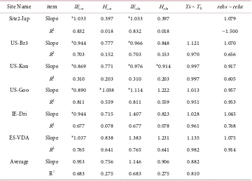
[image:14.595.194.554.406.664.2]3.6. Slope of Estimated against Observed in All Analyzed Data
Table 5 describes all analyzed daily data at tested six sites including observed and cor-rected versus estimated using the proposed method for lE and H as well as Ts versus T0
with rehs versus rehz. The feature is site specific. For corrected against estimated lE and H, the relationship is already described by Figure 5.
For lEobs versus lEest, IE-Dri and ES-VPA are overestimated (>15%). For Hobs versus
Hest, US-Goo and ES-VPA are overestimated while the other sites are underestimated.
(<±15%).
The Ts versus T0 relationship are strongly correlated for all sites. The relationship of
rehs versus rehz is also strong randomized at site-Jap and US-Br3, US-Kon remarkably
Table 5. All data analyzed by general method (general solution).
Site Name item lEcor Hcor lEobs Hobs Ts ~ T0 rehs ~ rehz
Site2-Jap Slope *1.033 0.397 *1.033 0.397 1.079
R2 0.832 0.018 0.832 0.018 −1.500
US-Br3 Slope *0.944 0.777 *0.966 0.848 1.121 1.070 R2 0.703 0.152 0.703 0.153 0.970 0.656
US-Kon Slope *0.869 0.771 *0.976 *0.914 0.997 0.917 R2 0.310 0.203 0.310 0.203 0.997 0.605
US-Goo Slope *0.890 *1.038 *1.114 1.222 1.013 0.957 R2 0.811 0.559 0.811 0.559 0.951 0.953
IE-Dri Slope *0.944 0.715 1.407 0.823 1.028 1.045 R2 0.677 0.078 0.677 0.078 0.961 0.768
ES-VDA Slope *1.037 0.838 1.383 1.231 1.135 1.075 R2 0.765 0.641 0.765 0.641 0.982 0.914
Average Slope 0.953 0.756 1.146 0.906 0.882 R2
0.683 0.275 0.683 0.275 0.810
Slope express the gradient of estimation (lEest, Hest) against correction (lEcor, Hcor) and observation (lEobs, Hobs), Initial
randomized.
3.7. Comparison of Estimated and Observed Evapotranspiration Rate
(
ETa
)
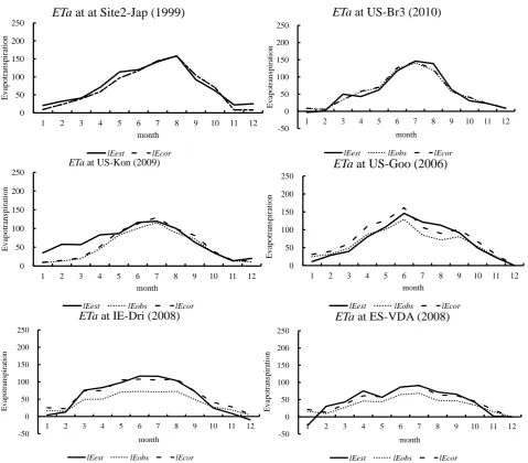
Using observed and estimated lE, monthly evapotranspiration was obtained at the all sites, as shown in Figure 7 by assuming 100 W∙m−2 equivalents for 3.53 mm∙day−1[12].
The initial value of rehs and constrains are chosen as aforementioned. If there are data gap in a given month, the monthly average ETa obtained as follows: The average ETa in a day multiplied the number of days of the month.
All sites describe very well reproduced the monthly change of ETa. In detail, al-though there are small differences between ETaobs, ETacor, and ETaestat all sites, the
[image:15.595.74.554.258.678.2]dif-ference was relatively small.
Figure 7. Comparison of observed (ETaobs) and estimated (ETaest) monthly evapotranspiration (mm∙month−1). Note: Initial
con-dition and constraints are the same with Figure 3. Observed data attached as reference.
0 50 100 150 200 250
1 2 3 4 5 6 7 8 9 10 11 12
E va pot ra ns pi ra ti on month
ETa
at at Site2-Jap (1999)
lEest lEcor -50 0 50 100 150 200 250
1 2 3 4 5 6 7 8 9 10 11 12
E va pot ra ns pi ra ti on month
ETa
at US-Br3 (2010)
lEest lEobs lEcor
0 50 100 150 200 250
1 2 3 4 5 6 7 8 9 10 11 12
E va pot ra ns pi ra ti on month
ETaat US-Kon (2009)
lEest lEobs lEcor
0 50 100 150 200 250
1 2 3 4 5 6 7 8 9 10 11 12
E va pot ra ns pi ra ti on month
ETa
at US-Goo (2006)
lEest lEobs lEcor
-50 0 50 100 150 200 250
1 2 3 4 5 6 7 8 9 10 11 12
E va pot ra ns pi ra ti on month
ETa
at IE-Dri (2008)
lEest lEobs lEcor
-50 0 50 100 150 200 250
1 2 3 4 5 6 7 8 9 10 11 12
E va pot ra ns pi ra ti on month
ETa
at ES-VDA (2008)
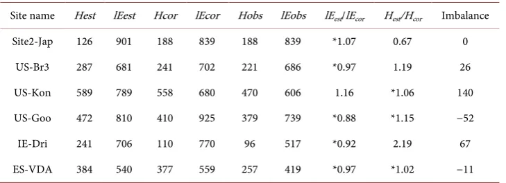
Besides the pattern of monthly changes, the total amount of the ETa issummarized in Table 6. The amount of annual lEestand Hest are satisfactorily consistent with lEcor
and Hcoror lEobs and Hobs, i.e., ETaest/ETacor (<±15%) excluding US-Kon. US-Kon has big
imbalance 140 mm∙year−1 even if after correction by regression analysis. The other sites
have a relatively small imbalance. The facts describe that ETa can be estimate by our method within 85% accuracy.
4. Consideration
4.1. Relationship of Penman Method with Proposed Method
To verify the validity of our method, our method was compared with penman method. Penman method is used to evaluate evaporation from the saturated or wet soil surface that corresponding to our proposed method as rehs equals to 100%.
Penman evaporation evaluated by Equation (14) [13]
(
10)
{
( ) ( )
}
0.26 1 0.537 sat
Rn
Ep U e Tz e Tz
γ λ γ
∆ ∆
= × + × × + × × −
∆ + ∆ + . (14)
Here, Δ is the slope of saturated vapor pressure curve (hP∙˚C−1) at Tz, γ is
hygros-copic constant (hP∙˚C−1), λ is latent heat flux (MJ∙kg−1), U
10 is wind speed at 10 m height
(m∙sec−1), another variable already described.
Figure 8 describes the comparison of evaporation estimated by Penman method with
[image:16.595.193.558.541.673.2]our proposed method using daily data of Ishikawa Prefectural Forest Experimental Sta-tion (Latitude (+N/−S): 36.4309, Longitude (+E/−W): 136.6424) (2014). The result by our method obtained using Equation (3) that optimized Ts at 100% of rehs reproduced well Penman’s result even though a little scattered. The scattered point may produce with observation quality by related climate elements. Our method does not require the wind speed correction that appeared in the second term of right hand side in Penman Equation (14), which was already pointed out by Urano [13]. In addition, constraint of Rn – G > lE and H is applied.
Table 6. Total amount of evapotranspiration estimated and observed including correction (mm∙year−1).
Site name Hest lEest Hcor lEcor Hobs lEobs lEest/lEcor Hest/Hcor Imbalance
Site2-Jap 126 901 188 839 188 839 *1.07 0.67 0
US-Br3 287 681 241 702 221 686 *0.97 1.19 26
US-Kon 589 789 558 680 470 606 1.16 *1.06 140
US-Goo 472 810 410 925 379 739 *0.88 *1.15 −52
IE-Dri 241 706 110 770 96 517 *0.92 2.19 67
ES-VDA 384 540 377 559 257 419 *0.97 *1.02 −11
Figure 8. Comparison of Penman method with our method (W∙m−2).
4.2. Comparison of Bulk Transfer Method at Wetted Soil Surface with
our Method
Furthermore, to obtain more reasonable result, we applied the Bulk Transfer Concept (BTC). The heat balance equation of the BTC can be expressed as Equation (15) [14]. The third term of left hand of the equation expressed the sensible heat flux and the fourth term expressed the latent heat flux. Before optimization, Equation (15) is not closed because CH, CE and Ts are assumed. The optimization conducted as the ε goes to
minimum.
(
)
0.622( ) ( )
P H E
Rn G C C Ts Tz Uz l C e Ts e z Uz
P
ρ ρ ε
− − − − − =
. (15)
Here, CH is bulk transfer coefficient of sensible heat flux, CE is bulk transfer
coeffi-cient of latent heat flux, Uz is wind speed, other variables already described.
As described in Figure 8, our method using Equation (15) with the condition of CH=
CE, that is the same of Penman method’s assumption [14], is very well reproduced,
al-though the procedure does not unified the variables CH= CE and Ts mathematically
because one equation determine two variables.
4.3. Comparison of Observed
Ts
with Estimated by Radiometer
Ts
To verify the reasonability of estimated Ts, Figure 9 compares the estimated Ts with observed Ts by radiometer at three sites. The sites almost indicate well coincident with each other, thus, the data shows the validity of the Ts estimation.
5. Discussion
5.1. Initial Values and Constraints
There are plural results i.e., local minimum, as satisfying Equation (8) and Equation (9) at different initial values because of nonlinear simultaneous solution. One of the tech-nical points of our research is how to find out the reasonable initial values of Ts and
y = 1.003x R² = 0.972
-2 -1 0 1 2 3 4 5 6 7 8
-1 0 1 2 3 4 5 6 7 8
O
ur
m
ethod by
B
ulk
tr
ansf
er
Penman method
Penman versus Our method by bulk transfer method (2010-2013.5)
y = 0.932x R² = 0.823
-2 -1 0 1 2 3 4 5 6 7
-2 -1 0 1 2 3 4 5 6 7
O
ur
m
ethod
by
B
ow
en r
atio c
onc
ept
Penman method
Figure 9. Comparison of Ts observed by radiometer and estimated (˚C).
rehs with constrains. We approach the final values of rehs and Ts from both sides satu-rated and observed rehz with constraints of b < 0 or b > 0. The results obtained by this procedure are mostly successful. One important thing is that the initial values Ts and rehs to be set as possible as vicinity to the final values.
5.2. Abnormal Fluctuation of
B
app(Singularity of
B
app)
If Ts approaches zero in convergence process, Bappis remarkably increased according to
approaching zero from the opposite side, positive and negative, as shown in Figure 10. This tendency is almost independent of
(
Ts Tz−)
, although there are small differences.Actually, when denominator of Equation (4) approaches zero q T
(
s ass,)
=q T( )
z i.e.,rehs approaches to
( )
( )
1sat sat
rehz×q Tz ⋅q Ts − , the abnormal Bappappeared. To avoid
this conflict, Bapp is limited to (−100 < Bapp< 100) as aforementioned, referring to the
observed and calculated data approximately [1].
6. Conclusions
In the natural world, the air temperature and humidity reflect the partitioning of sensi-ble and latent heat flux from Rn and G. Based on this concept, we attempt to estimate H
y = 1.028x
R² = 0.666
0 10 20 30 40 50
0 10 20 30 40 50
T
s e
st
TsObserved by long wave radiation
Ts
long waveversus
Ts
estat US-Br3
y = 1.180x
R² = 0.966
0 10 20 30 40 50
0 10 20 30 40 50
T
s e
st
TsObserved by long wave radiation
Ts
long waveversus
Ts
estat US-Goo
y = 1.100x
R² = 0.914
0 10 20 30 40 50
0 10 20 30 40 50
T
s e
st
TsObserved by long wave radiation
Figure 10. Relationship between Bapp and temperature Ts when Ts − Tz = 1.0˚C [1].
and lE reciprocally using single height temperature and humidity, and Rn and G by ap-plying the Bowen ratio concept on the soil surface. This feature can be remarkably ex-tended to the field of utilization. The unknown variables Ts and q Ts
( )
(i.e., rehs) areestimated by an optimization procedure as satisfying heat balance relationship. The va-lidation of the method was achieved by the six sites in the humid regions of Japan, USA and Europe. lE and H were observed by the eddy covariance method at these sites, ex-cept lE in Japan site. Analysis is conducted on an hourly basis and summarized daily. The main results are as follows:
1) The hourly and yearly change of the estimated lE and H very well coincided with the observed values at all sites.
2) The estimated lE and H versus corrected lE and H or observed lE and H are satis-factory coincided.
3) The hourly change of Ts and rehs can be estimated by the method that is very dif-ficult to observe at actual site.
4) The estimated evaporation ETa satisfactorily coincided with corrected and ob-served ETa not only monthly change but also annual amount.
5) The method compared with penman method and confirmed the validity.
The estimated results have not completely reproduced the observations, but the re-sults are mostly satisfactory. This fact shows that the method is useful for the estima-tion of lE and H. The remarkable feature of the new method is that it is applicable for the approximate of lE and H using a single height of Tz and rehz with Rn and G. For estimation of ETa, this method will be applicable to various local areas because of re-quired data easily obtained.
But, there are problems that still remain. The error plain i.e., εi in Equation (3)
re-lated to Ts and rehs, is very complicated because of nonlinear simultaneous equation having many local minimum. Therefore, the selection of initial values of Ts and rehs is important issue to be solved in future. On the other hand, this research is restricted at humid region but analysis of sensible and latent heat flux at arid and semi-arid region is
0.0E+00 5.0E-05 1.0E-04 1.5E-04 2.0E-04 2.5E-04 3.0E-04 3.5E-04 4.0E-04 4.5E-04
-8.0 -6.0 -4.0 -2.0 0.0 2.0 4.0 6.0 8.0
-3.0 -2.0 -1.0 0.0 1.0 2.0 3.0
q
sat
(
Ts
)-q
sat
(
Tz
)
Bapp
Ts
Bapp
also very important. This is also another big problem to be solved in future.
We conclude that the partitioning of lE and H is controlled by energy conservation in nature. Realistically, the observed temperature and humidity are strongly affected by the partitioning of H and lE, and vice versa. Therefore, using the observed temperature, humidity and common climate elements, the lE and H values are reciprocally approx-imated by the optimized techniques.
Acknowledgements
We sincerely thanks for providing the AmeriFlux and EuroFlux principal investigation for data accessed on July 5, 2015. We sincerely thank Dr. Asanuma Jun, a professor at Tsukuba University, for providing valuable data for the eddy covariance method; Dr. Kuwagata Tsuneo, Dr. Fujihara Yoichi and Dr. Takimoto Hiroshi for providing valua-ble comments on the optimization procedure. We also thank Dr. Yoshida Masashi and Dr. Noto Fumikazu, who are staff members at Ishikawa Prefectural University, for re-cording the data. We also thank the staff at the Ishikawa Forest Experiment Station.
References
[1] Maruyama, T. and Segawa, M. (2016) Reciprocal Analysis of Sensible and Latent Heat Fluxes in a Forest Region Using Single Height Temperature and Humidity Based on the Bowen Ratio Concept. Journal of Water Resource and Protection, 8, 724-742.
http://dx.doi.org/10.4236/jwarp.2016.87059
[2] Kondo, J. (1996) Meteorology on Water Environment, 6. Water and Heat Balance on Soil Surface. Asakura Publishing Ltd., Tokyo, 128-159.
[3] Twine, T.E., Kustas, W.P., Norman, J.M., Cook, D.R., Houser, P.R., Meyers, T.P., Prueger, J.H., Staks, P.J. and Wesely, M.L. (2000) Correcting Eddy-Covariance Flux under Estimates over a Grassland. Agricultural and Forest Meteorology, 103, 279-300.
http://dx.doi.org/10.1016/S0168-1923(00)00123-4
[4] Wison, K., Goldstein, A., Falge, E., Abbinet, M., Baldocchi, D., Berbingier, C., Ceulemans, R., Dolman, H., Field, C., Grelle, A., Ibrom, A., Law, B., Kowalski, A., Meyers, T., Mon-crieff, J., Monson, R., Oechel, W., Tenhunen, J., Valentini, R. and Verma, S. (2002) Energy Balance Closure at FLUXNET Sites. Agricultural and Forest Meteorology, 113, 223-243. [5] Allen, R. (2008) Quality Assessment of Weather Data and Micrometeorological Flux Impact
on Evapotranspiration Calculation. Journal of Agricultural Meteorology, 64, 191-204.
http://dx.doi.org/10.2480/agrmet.64.4.5
[6] Asanuma, J. (2012) Site2-Jap, Data of Heat and Water Balance Observation, 1999-2011 by CD. Center for Research in Isotope and Environmental Dynamics, Tsukuba University. [7] Prueger, J.H. (2010) Brooks Field Site 11 (US-Br3) AmeriFlux L2 Data.
http://cdiac.esd.ornl.gov/programs/ameriflux/data_system/aaBrooks_Field_Site_11_pf.html
[8] Brunsell, N. (2009) Konza Prairie (US-KON) AmeriFlux L2 Data.
http://cdiac.esd.ornl.gov/programs/ameriflux/data_system/aaKonza_Prairie_pf.html
[9] Meyers, T. P. (2006) Goodwin Creek (US-Goo) AmeriFlux L2 Data.
http://cdiac.esd.ornl.gov/programs/ameriflux/data_system/aaGoodwin_Creek_pf.html
[10] Carrara, A. and Gimeno, C. (2008) Vall dAlinya (ES-VDA) European Fluxes Database Cluster L2 Data.
Clus-ter L2 Data.
[12] Kondo, J. (2015) Heat Balance and Climate on Soil Surface.
[13] Urano, S.-I. (2012) Study on Bowen ratios in the Penman and Priestly·Taylor Equations.
Geophysical Bulletin of Hokkaido University, Sapporo, 15, 91-107
Appendix 1
The GRG Nonlinear Solving Method for nonlinear optimization: developed by Leon Lasdon (University of Texas at Austin) and Alan Waren (Cleveland State Universi-ty) and enhanced by Frontline Systems, Inc.
For more information about the other solution algorithms, advice on building effec-tive solver models, and solving larger scale problems, contact: Frontline Systems, Inc.
Web site: http://www.solver.com, E-mail: info@solver.com
Estimated results have not completely reproduced the observations, but the results are mostly satisfaction.
Appendix 2
Using modules of Visual Basic for Applications (VBA) in the manuscript Sub Macro “Number1 ()
' Macro ”Number 1”:GRG method
Dim r As Long Dim lastRow As Long
lastRow = Range(“〈Column Alphabet〉” & Rows Count).End (xlUp).Row
SolverReset
For r = 〈Start row number〉 To 〈End row number〉
SolverReset
SolverOptions Precision:=0.000001, Convergence:=0.0001, StepThru:=False, Scaling:=False _
, AssumeNonNeg:=False, Derivatives:=2
SolverOk SetCell:= "Row" & r, MaxMinVal:=2, ValueOf:=0_
, ByChange:=Range(Cells(r, 〈First column number〉), Cells(r, 〈Last column
number〉))
SolverAdd CellRef:="$ 〈rehs’s Column Alphabet〉" & r, Relation:=1,
Formula-Text:=1
SolverAdd CellRef:="$ 〈rehs’s Column Alphabet〉" & r, Relation:=3,
Formula-Text:=0
SolverAdd CellRef:="$ 〈RTs’s Column Alphabet〉" & r, Relation:=1, FormulaText:=5
SolverAdd CellRef:="$ 〈RTs’s Column Alphabet〉" & r, Relation:=3, FormulaText:=
-5
SolverAdd CellRef:="$ 〈H estimated’s Column Alphabet〉" & r, Relation:=1,
For-mulaText:= "$ 〈Rn-G observed’ s Column Alphabet〉$ &r
SolverAdd CellRef:="$ 〈H estimated’s Column Alphabet〉" & r, Relation:=3,
For-mulaText:=-100
SolverAdd CellRef:="$ 〈LE estimated’s Column Alphabet〉" & r, Relation:=1,
FormulaText:= "$ 〈Rn-G observed’ s Column Alphabet〉$ &r
SolverAdd CellRef:="$ 〈LE estimated’s Column Alphabet〉" & r, Relation:=3,
FormulaText:=-100
Formula-Text:=100
SolverAdd CellRef:="$ 〈Bapp’s Column Alphabet〉" & r, Relation:=3, FormulaText:=
-100
※in case of b>0
SolverAdd CellRef:="$ 〈b estimated’s Column Alphabet〉" & r, Relation:=3,
For-mulaText:=0 ※in case of b<0
SolverAdd CellRef:="$ 〈b estimated’s Column Alphabet〉" & r, Relation:=1,
For-mulaText:=0
SolverSolve UserFinish:= True, ShowRef:="DummyMacro" Next
End Sub
Submit or recommend next manuscript to SCIRP and we will provide best service for you:
Accepting pre-submission inquiries through Email, Facebook, LinkedIn, Twitter, etc. A wide selection of journals (inclusive of 9 subjects, more than 200 journals)
Providing 24-hour high-quality service User-friendly online submission system Fair and swift peer-review system
Efficient typesetting and proofreading procedure
Display of the result of downloads and visits, as well as the number of cited articles Maximum dissemination of your research work
Submit your manuscript at: http://papersubmission.scirp.org/