Long memory and structural breaks in time series models

Long Memory and Structural Breaks

in Time Series Models

Stepana Lazarova

Ph.D. Thesis

Department of Economics

London School of Economics and Political Science

UMI Num ber: U 2 2 2 0 8 1

All rights r e serv e d

INFORMATION TO ALL U S E R S

T h e quality o f this reproduction is d e p e n d e n t upon th e quality of th e c o p y su bm itted .

In th e unlikely e v e n t that th e author did not s e n d a c o m p le te m an u scrip t

and th ere are m issin g p a g e s , t h e s e will b e n oted . A lso , if m aterial had to b e rem oved , a n ote will ind icate th e d eletio n .

Dissertation Publishing

UMI U 2 2 2 0 8 1

P u b lish ed by P ro Q u est LLC 2 0 1 4 . C opyright in th e D isserta tion held by th e Author. Microform Edition © P ro Q u est LLC.

All rights r e se r v e d . T his work is protected a g a in s t u nau th orized cop y in g under Title 17, United S ta te s C o d e .

P ro Q u est LLC

7 8 9 E a st E ise n h o w e r Parkw ay P.O. B ox 1 3 4 6

This thesis has been subm itted to the University of London in partial fulfil­ ment of the requirements for the Ph.D. degree in Economics at the London School of Economics and Political Sciences (LSE).

No part of this doctoral dissertation had been presented to any university for any degree.

Chapter 3 was undertaken as joint work with Professor Javier Hidalgo.

Stepcina Lazarovd

A bstract

This thesis examines structural breaks in time series regressions where both regressors and errors may exhibit long range dependence. Statistical proper­ ties of methods for detecting and estimating structural breaks are analysed and asymptotic distribution of estimators and test statistics are obtained. Valid bootstrap methods of approximating the limiting distribution of the relevant statistics are also developed to improve on the asymptotic approxi­ mation in finite samples or to deal with the problem of unknown asymptotic distribution. The performance of the asymptotic and bootstrap methods are compared through Monte Carlo experiments. A background of the concepts of structural breaks, long memory and bootstrap is offered in Introduction where the main contribution of the thesis is also outlined. Chapter 1 proposes a fluctuation-type test procedure for detecting instability of slope coefficients. A first-order bootstrap approximation of the distribution of the test statistic is proposed. Chapter 2 considers estimation and testing of the time of the

C ontents

Introduction 8

1 Testing for structural change in regression w ith long m em ory

processes 21

1.1 In tro d u ctio n... 21

1.2 Model and asymptotic r e s u l t s ... 22

1.3 Bootstrap p r o c e d u re ... 34

1.4 Finite sample p r o p e rtie s ... 39

1.5 C o nclusions... 41

l.A P r o o f s ... 44

1.B L e m m a s ... 47

2 Locating structural change in regression w ith long m em ory processes 75 2.1 In tro d u ctio n... 75

2.2 Linear regression with b r e a k ... 78

2.3 Asymptotic properties of the breakpoint and slope estimator . 81 2.4 Hypothesis t e s t i n g ... 8 6 2.5 Weak b re a k s... 8 8 2.6 Bootstrap under shrinking b re a k ... 90

2.7 Finite sample p r o p e rtie s ... 93

2.8 C on clu sio n s... 95

2.A P r o o f s ... 99

3 Inference on th e tim e o f break in regression w ith long m em ory

processes 138

3.1 In tro d u ctio n ... 138

3.2 Bootstrap under fixed b r e a k ... 141

3.3 Asymptotic properties of the bootstrap p ro c e d u re ... 148

3.4 C on clu sio n s... 152

3.A P r o o f s ... 155

3.B L e m m a s ... 165

List o f Tables

1.1 Detecting a break: Size of the bootstrap and asymptotic tests 42 1.2 Detecting a break: Rejection probabilities of the bootstrap and

asymptotic tests under the alternative h y p o th e s is ... 43

2.1 Locating a break: Size of the bootstrap and asymptotic tests . 96 2 .2 Locating a break: Rejection probabilities of the bootstrap and

Acknowledgem ent s

I would like to thank Javier Hidalgo for his generous supervision during my doctoral studies at LSE, for the key contribution to a part of the thesis, and for inspiring me by having a high expectation of me since the beginning. I have also received advice and encouragement from Liudas Giraitis, Oliver Linton and Peter Robinson, for which I am very grateful.

Thanks also go to my friends and colleagues at the Department of Eco­ nomics, in particular Jesiis Maria Carro, David Jacho-Chdvez, Xiaohong Chen, Piotr Eliasz, Javier Hualde, Fabrizio Iacone, Dennis Kristensen, Jos6 Sanz- Vidal, Marcia Schafgans and Ayan Sen, for making my years at LSE an en­ joyable experience.

During my doctoral research and in the years leading to it, I greatly bene­ fite d from stimulating discussions with Anindya Banerjee, Robert Chirinko, Saul Estrin, Paul Geroski, Stephen Hall, Marie HuSkovd, Chihwa Kao, Pietro Muliere, Lorenzo Trapani and Fabio Trojani. Special thanks to Giovanni Urga for his continuous encouragement and support.

I gratefully acknowledge financial support from the Dennis Sargan Memo­ rial Fund and from the Economic and Social Research Council through grants R000238212 and R000239936. My studies were also made possible by the financial assistance through the following scholarships: Royal Economics So­ ciety Junior Fellowship, LSE Research Studentship, Department of Economics Award (LSE), Overseas Research Studentship, CK Hobson Scholarship (LSE) and British Council Chevening Scholarship.

Introduction

This thesis examines structural breaks in time series regressions. The main contribution to the literature in the field is twofold. First, statistical proper­ ties of methods for detecting and estimating structural breaks are analysed when both regressors and errors are allowed to exhibit long range dependence. Second, valid bootstrap methods of approximating the limiting distribution of relevant estimators are developed under possible long range dependence.

The principal keywords of the thesis are structural breaks, long memory and bootstrap. The following sections offer some background notes on these concepts and explain in what way this thesis adds to the body of knowledge in respective fields. The last section outlines the notation used throughout the thesis.

Structural breaks

Structural stability is a desirable property of any econometric model. Models th at are structurally unstable tend to lead both to erroneous in-sample analy­ sis and out-of-sample forecasts. Tests of parameter instability and structural change have therefore been a subject of a large body of statistical and econo­ metric literature. The maintained hypothesis of parameter stability has been tested against both specific and general forms of alternative hypothesis.

estimates, as in the fluctuation tests of Sen (1980) or Ploberger et al. (1989). Alternatively, parameter stability tests can be designed against a specific alternative. Example of specific alternatives are one-time change in para­ meters as in the papers by Quandt (1960) or Andrews (1993), or parameters following random walk (Nyblom (1989)). Though constructed to detect a spe­ cific parameter behaviour, these tests are usually shown to have power against a broader range of departures from the null of parameter constancy.

Beside specification testing, the presence or absence of structural stability may be of interest in itself. If a structural change is detected, an inquiry into the character of the change may reveal factors that caused the structural shift and may lead to a successful revision of the original model. A prime example of this is the article of Perron (1989) who argues that many key economic variables should be modelled as stationary around a deterministic trends with breaks. Such models imply that the majority of shocks in economy are transitory and only few shocks have a permanent effect. The structural break model of Perron is an answer to the stochastic trend model of Nelson and Plosser (1982) which imply th at all random shocks have a permanent effect on the economy. The work of Perron brought a change in the common view of the nature of dynamics of economic variables and inspired further investigation of instability in economic systems.

When it is known th at the parameters of a model undergo a break, the knowledge of the date of break is often relevant to researchers, for exam­ ple when judging a delay in reaction of agents to a change in economic pol­ icy. There is a steadily growing body of literature on estimating the time of change. Hinkley (1970), Yao (1987) and Bhattacharya (1987) deal with max­ imum likelihood estimation of time of a shift in mean of otherwise identically distributed independent observations. In the context of dependent observa­ tions, Bai (1994, 1997b) allows for a linear process with short memory while Bai (1997a), Bai and Perron (1998) and Fiteni (2002, 2004) analyse estima­ tors of the time of break in parameters of linear regression model with mixing data.

and locating structural change. More specifically, the size of change is assumed to decrease with increasing sample size. Examples of articles that adopt this assumption are Ploberger et al. (1989) and Andrews (1993) for detecting the structural change and Picard (1985) and Bai and Perron (1998) for estimating the date of break.

In the context of testing for parameter instability, this assumption may be regarded as innocuous since it can be argued th at if a test procedure is capable of detecting small changes in the structure of the model, it will also be capable of detecting large changes. However, in the context of estimating the date of break, the assumption is no longer incontroversial. The gain in information due to the increase in the sample size is not sufficiently large to offset the loss of information due to the decrease in the magnitude of the break. The dispersion of the breakpoint estimator grows to infinity and tests of hypotheses about the date of change against fixed alternatives lose power in growing samples.

The only solution to this problem is to model the break as having a fixed size. Under the fixed break assumption, however, the limiting distribution of the location estimator depends on the distribution of the data and is therefore generally unknown and unavailable for the purposes of statistical inference. Hinkley (1970) attempts to circumvent the problem of intractability by as­ suming that the distribution of data is known. His method is difficult or impossible to implement in any but the most simple settings and in any case the assumption that the distribution of data is known is unrealistic. Since then, attempts to reconcile the advantages in assuming fixed breaks with the need for a tractable asymptotic distribution have been largely abandoned, with an exception of Antoch et al. (1995) who devise a bootstrap method for regression with independent identically distributed errors.

The current state of the research on structural changes in linear models with time series has been reviewed by Banerjee and Urga (2005) and Perron (2006). Other overviews of the work on structural breaks include the article by Stock (1994) and the special issue of the Journal of Econometrics on "Recent developments in the econometrics of structural change" edited by Dufour and Ghysels (1996).

dependence on estimators of time of break has been examined by Antoch et al. (1995, 1997), Horvath and Kokoszka (1997) and Kuan and Hsu (1998) in the framework of linear processes with a break in mean. Hidalgo and Robinson (1996) propose tests for a change in parameter values at a known time point in linear regression models with long-memory errors while Hidalgo (2003b) designs a test for the presence of breaks in nonparametric regression function with possibly strongly dependent errors.

T his thesis

This thesis examines stability of slope coefficients in the linear regression model. An important distinction from the majority of existing literature is th at we allow both regressors and errors to be possibly long range depen­ dent. We are interested in two aspects of the problem of parameter stability. First, we examine methods of detecting structural instability and estimating the date of structural change. Second, we analyse in some detail the effect of the assumed size of break on statistical properties of estimators and test statistics, and attem pt to resolve the difficulties arising from the imposition of the standard assumption of shrinking breaks.

Chapter 1 proposes a fluctuation-type method of testing for structural sta­ bility. The procedure is based on a process of least-squares slope coefficient estimators. The fluctuation of the process is measured by a continuous func­ tional and the presence of instability is indicated by large fluctuation. Though the test is constructed to have power against the alternative of a structural break, it is shown to be powerful against a broader range of alternatives, such as multiple breaks, smooth transition between two steady levels of parameters and a continual change of parameter. The functional defining the test statistic can be chosen to reflect beliefs about the form of alternative and so improve the power of the test procedure.

long memory time series, fractional Brownian motion processes are usually expected to appear in expressions describing the asymptotic distribution. In our stochastic regressor framework, the effect may be viewed as a mutual sto­ chastic dampening of regressors and errors where the individual series may exhibit long memory but their product displays short memory.

In Chapter 2, we examine a least squares method of estimating the time of

the break. Here again the results from the short memory literature carry over to our long memory setting under the assumption of a break of both fixed and shrinking size. The magnitude of break, however, turns out to be crucial in determining the qualitative properties of the asymptotic distribution of the breakpoint estimator. One of the main contribution of Chapter 2 is therefore

an analysis of the asymptotic behaviour of the estimator under various as­ sumptions on the size of break, ranging from a fixed size of break through a size shrinking at a certain rate to zero size. While the assumptions of fixed and shrinking breaks have been examined in a variety settings with short memory data, and we extend the analysis to the long-memory time-series regression setting, the assumption of a weak break, that is break of a rapidly decreasing size, has not been analysed yet in the literature.

The conclusion is th at when the size of the break is fixed, the asymptotic distribution depends on the entire joint distribution of the regressors and the error term. When the size of the break is shrinking but more slowly than the square root of the sample size, the asymptotic distribution of breakpoint is free of nuisance parameters and is explicitly known. When the size of the break is shrinking faster than the square root of the sample size, or when there is no break in the data generating process, the question of estimating the location of the break becomes vacuous because in this circumstance the break is not detectable. In the borderline case of the size of break decreasing with exactly the square root of the sample size, the break can be detected but there is insufficient information for estimating its location.

ution is called for. One such procedure, based on the bootstrap, is proposed in Chapter 3.

Long m em ory

The phenomenon of the slow decay of correlation between observations that are far apart had been observed in various scientific fields since well over one hundred years ago. One of the first important statistical treatments of long memory has been in hydrology by Hurst (1951) who considered the reseeded adjusted range statistic and found its behaviour inconsistent with short range dependence assumption. In economics, one of the first to observe the long- memory properties of economic time series has been Adelman (1965) who observed peaks of estimated spectral functions around zero frequency. The peaked spectral density has been claimed by Granger (1966) to be the typical spectral shape of an economic variable.

For stochastic processes, the property of possessing long memory has been variously defined through the behaviour of the autocorrelation function as hav­ ing hyperbolically decaying autocorrelations or having autocorrelations that are nor absolutely summable, through the behaviour of the spectral density as having a pole at zero frequency, or through the behaviour of the partial sums of the process as having variance that is increasing faster than the sample size. These definitions are closely related but not equivalent.

The degree of memory of a process may be described by the parameter

d which we take to be the order of the singularity of the spectral density at zero. Estimation of d is a well-researched topic and a wide array of esti­ mators is available to practitioners. Recent surveys of developments in long memory estimation and testing include Robinson (2003) and Banerjee and Urga (2005). Various results are collected in surveys by Robinson (1994a) and Baillie (1996), in a book by Beran (1994) and in a recent special issue of the Journal of Econometrics on "Long Memory and Non-Linear Time Series" edited by Davidson and Terasvirta (2002).

(Diebold and Inoue (2001)), processes with certain type of deterministic trend (Bhattacharya et al. (1983)), error duration processes (Parke (1999)) and, importantly from our point of view, processes with structural breaks (Engle and Smith (1999) and Granger and Hyung (2004)). Accordingly, there is a growing body of literature on distinguishing genuine long memory time series from those with other features (Ktinsch (1986), Shimotsu (2005) and Berkes et al. (2006)).

There is also work that nests both long memory and some of the above features, but focuses on the analysis of one feature only. Iacone (2006) ex­ amines the degree of memory of a given series with possible presence of the nuisance deterministic components including broken trends. In the opposite direction, Hidalgo and Robinson (1996) allow for the presence of long mem­ ory but regard it as a nuisance phenomenon and concentrate on testing for structural breaks in the framework of linear regression. A similar approach is taken in articles by Antoch et al. (1995, 1997), Horvath and Kokoszka (1997) and Kuan and Hsu (1998) mentioned in the previous section.

This thesis

In this thesis, we are interested in structural breaks and view long memory as a nuisance. Our aim is to develop methods in which the user does not need to know the degree of memory of the data, as long as the data are stationary. As a result, we do not discuss the estimators of the long memory parameter and we only use the existing estimators.

In Chapters 1 and 2, we show th at the classical least squares methods for

detecting and locating breaks, devised originally under the assumption of no or short memory in regressors and errors, can be used without change under long memory, and the degree of memory does not need to be estimated. We also show that the statistical properties of the estimators remain unchanged. The only place where an allowance for possible presence of long memory needs to be made is when the user wishes to conduct a bootstrap test since it seems convenient to carry out the bootstrap procedure in the frequency domain.

researcher uses the local Whittle estimator proposed by Robinson (1995b) and we show its consistency when the underlying series is replaced by residuals.

B o o tstr a p

When the distribution of an estimator or a test statistic is unknown or if it is difficult to calculate, it can be approximated by the bootstrap. Bootstrap methods can also be used to provide more accurate approximation of the finite sample distribution than the approximation obtained from first order asymptotic theory.

The core idea of the bootstrap is to replace the unknown distribution of a random variable by the empirical distribution of a random sample drawn from th at distribution. However, when the data are not independent and identically distributed, the basic bootstrap of Efron (1979) is not valid and the bootstrap procedure needs to be modified to reflect the dependence or heterogeneity structure of the data. In the time series context, an early adaptation of the basic bootstrap method rests on the assumption th at the data are generated by a finite-order stationary ARMA process with independent identically dis­ tributed innovations (Freedman (1984), Efron and Tibshirani (1986)). In a direction towards nonparametric methods, Btihlmann (1997, 1998) approxi­ mates the linear infinite-dimensional process by a sieve of finite-dimensional autoregressive processes whose order is growing with the sample size. Diebold et al. (1998) propose a purely nonparametric bootstrap method based on the Cholesky factorization.

A different way of approximately preserving the temporal dependence structure of the data is to resample blocks of data. Carlstein (1986) and Ktinsch (1989) propose to resample nonoverlapping and overlapping blocks of data, respectively, and to concatenate the blocks to generate a bootstrap sam­ ple. Politis and Romano (1992) introduce an idea of subsampling, regarding blocks of data - subseries - as new pseudo-samples.

time-series bootstrap can be highly sensitive to the choice of the dimension parameter, particularly in samples of moderate size. Although automatic procedures for choosing the dimension have been devised for some methods, they can be computationally expensive.

Nonparametric bootstrap procedures can alternatively be carried out in the frequency domain where either frequency domain data, that is the dis­ crete Fourier coefficients, or their squares, th at is the periodograms, can be bootstrapped. This approach is motivated by the observation th at converting a stochastic process from the time domain to the frequency domain reduces serial correlation of the process though it induces heteroskedasticity. Boot­ strap method of Ramos (1988) for Fourier coefficients or Franke and Hardle (1992) and Dahlhaus and Janas (1996) for periodograms require a consistent estimate of the spectral density and therefore a choice of a bandwidth. Local periodogram bootstrap of Paparoditis and Politis (2000) avoids the need for estimating the spectrum but again demands a bandwidth choice.

Hidalgo (2003a) proposes a method that eliminates the choice of lag length or bandwidth. He suggests to bootstrap OLS residuals in frequency domain. His bootstrap procedure is easy to implement and computationally inexpen­ sive. His approach is the only one among the methods cited so far th at has been shown to be valid for strongly dependent data.

This thesis

One of the goals of this thesis is to design bootstrap procedures th at are valid for short as well as long memory time series. As with parameter estimation, we aim to avoid the need for the researcher to know or estimate the degree of memory of the data, as long as the data are stationary. We first propose a bootstrap procedure that is useful for approximation of the distribution both of test statistics for detecting the break in Chapter 1 and of the estimator of

the date of break under shrinking break in Chapter 2.

heteroskedasticity is accounted for by re-scaling the resampled values.

The procedure is essentially th at of Hidalgo (2003a). However, to prove the validity of the method in the context of time series regression with structural breaks, it is necessary to show that the method is successfully estimating not only the distribution of the normalized sum of a time series, but also the distribution of the entire process of its partial sums. The relevant concept here is the bootstrap weak convergence of Gin6 and Zinn (1990). The proof

of bootstrap weak convergence of the partial-sum process is one of the main contributions of the thesis.

The proposed procedure inherits the advantage of the original method of Hidalgo (2003a) of not requiring a user-chosen parameter such as the block length in the block bootstrap of Carlstein (1986) or the lag length in the sieve bootstrap of Btihlmann (1997, 1998).

While the bootstrap inference procedure in Chapters 1 and 2 is an op­

tional and advantageous alternative to asymptotic inference procedures, in Chapter 3 the limiting distribution of the breakpoint estimator depends on the unknown joint distribution of data and the use of the bootstrap or some other estimating procedure becomes a necessity if inference is to be carried out. The bootstrap procedure proposed in Chapters 1 and 2 asymptotically

matches the covariance structure of the underlying process. The ability to esti­ mate the second moment dependence structure is sufficient for approximating distributions th at are entirely described by the second-order structure, for ex­ ample the Gaussian distribution. However, it does not suffice for estimating a general joint distribution of a process.

In Chapter 3, we therefore design a more refined bootstrap method. The idea behind the bootstrap procedure is to fractionally difference the series in question and to approximate the resulting short memory process by an autoregressive process. The values to be resampled here are the estimated innovations of the process, and the bootstrap sample is created by refiltering and fractionally integrating the resampled innovations.

ical spectral decomposition of a smoothed estimate of the spectral density corresponding to the differenced process.

In contrast to the bootstrap procedure in Chapters 1 and 2, estimation of d

cannot be avoided though d remains a nuisance parameter. Moreover, the user needs to choose a bandwidth parameter for smoothing and a number of lags of the truncated linear process. Interestingly, however, it turns out th at the two parameters are directly related so that effectively the user chooses only one bandwidth parameter, and the value of this parameter can be determined by a cross-validation procedure. In return for the additional user input, the bootstrap delivers approximation of finite-dimensional joint distributions of the process.

To our knowledge, there is currently no bootstrap procedure available th at approximates the joint distribution of data while allowing for strong serial dependence. Construction of such a bootstrap procedure is therefore one of our main contributions to the literature.

N o ta tio n

Throughout the thesis, W denotes a p-dimensional vector of independent stan­ dard Brownian motion processes on [0,1] or on a set A C (0,1), ”= ^ ” de­

notes weak convergence in the space D (A)p of p-vectors of right-continuous functions with left-hand limits, endowed with the uniform metric p (x ,y ) = supreA \\x(t) — y(t )|| for x ,y € D (A)p. The statement yr ~ x t is equivalent

to the statement ^ —> 1 as T —> oo. For cr-algebras T , Q, T M Q is their union, that is the smallest cr-algebra containing all elements of T and Q.

For any real numbers a and 6, aVb = max {a, 6} and aAb — min {a, b}. For any integers j and A;, |j — k\+ = m ax{l, |j — fc|}. For a set S and a constant

a, S • a = {xa : x G S}. For nonnegative numbers I, m,

i,m, H t = i + i a t I

y at = <0 I = m,

, E t= m + 1 I > m.

[•] signifies integer part and I (•) is the indicator function of a set.

For a Hermitian matrix A, Amin (A) and Amax (^4) denote the smallest and the largest eigenvalue of A, respectively. Inequalities A > B and A > B

among two matrices hold if all the eigenvalues of A — B axe nonnegative and positive, respectively. For any matrix A, ||*|| denotes the maximum-eigenvalue norm, th at is \\A\\ = sup||x ||=1 ||A:r|| = A^ a2Y {A!A). We have ||j4||2 < t iA 'A and due to the equivalence of norms also tiA !A < C ||^4||2 for a constant C > 0.

For a generic function </?, we denote <Pj = (Aj), where Aj = 27rj/T , j = 1 , . . . , T are Fourier frequencies. For sequences {at}J=1 and {bt}J=1 of p-dimensional vectors,

t « a ( A ) = - 1= = ^ a t e ’*A ) A € [ - 7 T , ?r] ,

v 2 t t T f r ?

is the discrete Fourier transform of {at} and

Iab(X) = Wa (A) w'b (A), A G [ - 7 r, 7r ] ,

is the cross-periodogram matrix of {at} and {bt}. Notation f vv is reserved for the spectral density of a process {vt}.

Starred notation in k*, u*, E*, Op* and similar refers to quantities condi­ tional on data, taken with respect to the corresponding bootstrap probability measure. In particular, notation P* distinguishes the probability conditional on the a-algebra T t V Qt- For example,

P* (l** - k\ < x) = P < x T t V G t) ■

Similarly, E*, var* and cov* denote expectation, variance and covariance con­ ditional on T t V Gt, respectively. For a random variable X and a sequence

{ X T} of random variables, the statement X t ^ X is equivalent to the state­ ment

P * ( X T < x ) ^ P { X < x ) a s T —to o

Y and a sequence of stochastic processes {Yt}, Yt => Y stands for the weak convergence in probabihty as defined by Gine and Zinn (1990).

Stochastic orders of magnitude op*, Op* are defined as follows. Let {y?T} be a sequence of positive finite numbers. We say that Xt = Op* (<pT) as T —► oo if and only if for every e > 0 and 77 > 0 there exist finite M and Tq such that

for all T > To,

P ( P * ( \ X T\ > MipT) >r j ) <e.

We say that Xt = op* {<pT) as T —►0 0 if and only if for every 77 > 0,

P * ( \ Xt\ > W t) = op( 1 ) .

It is easy to verify some useful relations for the orders of magnitude op* and

Op*. For example, op* (1) • Op (1) = op* (1) or op* (1) + op (1) = op* (1).

C hapter 1

T esting for structured change in

regression w ith long m em ory

processes

1.1

In trod u ction

Parameter instability and structural change have been a subject of a large body of statistical and econometric literature. The maintained hypothesis of parameter stability has been tested against both specific and general forms of alternative hypothesis. When employed as a model-diagnostic tool, stability tests are constructed against all possible functions describing the evolution of parameters over time. Such tests axe based on the behaviour of regression residuals, as in CUSUM tests of Brown et al. (1975) and Ploberger and Kramer (1990, 1992), or on the behaviour of parameter estimates, as in the fluctuation tests of Sen (1980) or Ploberger et al. (1989).

Alternatively, parameter stability tests can be designed against a specific alternative. Example of specific alternatives are one-time change in parame­ ters as in the papers by Quandt (1960) or Andrews (1993), or parameters following random walk (Nyblom (1989)). Though constructed to detect spe­ cific parameter behaviour, these tests are usually shown to have power against a broader range of departures from the null of parameter constancy.

gression model where both regressors and errors are allowed to be long range dependent. The main contribution of the chapter is twofold. First, the lim­ iting distribution of the test statistics considered in the literature is typically a functional of Brownian motion. It is shown th at this remains true for test statistics based on the slope coefficient estimator in linear model with station­ ary long memory series. Secondly, as an alternative to computing the critical values for the test statistic, a first-order bootstrap approximation of the dis­ tribution of the test statistic is proposed and the validity of the bootstrap procedure is shown.

The chapter is organized as follows. Section 1.2 describes the model and the hypotheses of interest and states distributional results for the test statistic. Section 1.3 proposes a bootstrap approximation of the testing procedure and shows its validity. Section 1.4 offers a Monte Carlo study of the small sample performance of the bootstrap testing procedure. Section 1.5 concludes. The proofs of the results stated in the text are gathered in Section l.A. Section l.B contains some auxiliary results.

1.2

M od el and a sy m p to tic resu lts

We are interested in testing for structural change in regression models with processes that may possess long memory. We consider the model

yt = a + (3'tx t + Wt, £ = 1 , . . . , T , (1.1) where yt is the observed dependent variable, a is an unknown intercept, f t is a p-dimensional vector of unknown parameters, x t is a p-dimensional vector of the explanatory variables and ut is an unobserved stochastic disturbance. Our hypothesis of interest is whether the parameter vector f t stays constant,

Ho: f t = (3 for some f t for all t = 1, . . . , T.

Test procedures for the hypothesis of structural stability of general models are based on test statistics th at can be written as

Z t = <f> ( E t ) ,

where Et is a stochastic process on [0,1] or its subset with values in the

space of right-continuous functions with left-hand limits and 0 is a continuous

functional. The process Et is based on an estimator of parameters of a given model and its form reflects the choice of the testing principle. For example, if

{et,P < t < T } is the sequence of cumulative recursive residuals from the OLS estimates of the model (1.1) under the null as in the CUSUM test procedure of Brown et al. (1975), the stochastic process Et can be defined as Et =

{Et (t) = e[TT\,p /T < r < l} . Further examples of processes considered in the literature are Wald-, LM- and LR-like test statistic processes of Andrews

(1993), CUSUM of squares process of Brown et al. (1975), OLS CUSUM process of Ploberger and Kramer (1992), OLS parameter estimates process of Ploberger et al. (1989) and Sen (1980) or MOSUM process of Chu et al.

(1994).

The functional (f ) measures the excess fluctuation of the process E t with

respect to its hypothesized fluctuation. Depending on the belief about the form of the alternative, the functional <f) can be chosen to obtain good power of the test. A functional widely used in literature is the supremum functional. The test statistic can also be based on the Lg-distance like Cram6r-von Mises

test statistic with q = 2. The range functional, th at is the difference between the maximum and the minimum of a function, can have power advantage over the supremum functional in detecting smaller fluctuations of a process which changes its sign, as argued by Kuan and Hornik (1995). The average exponential functional of Andrews and Ploberger (1994) is shown to enjoy asymptotic optimality with respect to a weighted average power criterion.

In this chapter, we base the test procedure on the OLS estimators of the coefficient 5 in the model

where

, X / Xt t < [tT] ,

zt = zt (r) = < . (1.3) I 0 otherwise,

where 8 is a p-dimensional vector of parameters and where r lies in a subset A

of ( 0 ,1). In the interest of clarity, the explicit notation of dependence of zt on

t is sometimes dropped in what follows. The choice A = ( 0 ,1) appears natural

but for technical reasons the set A needs to be restricted to have closure in

( 0 ,1). The grounds for the restriction are discussed after stating Theorem 1.2

and its Corollary 1.1 below. In addition to technical reasons, there may be other motives for restricting the set A away from ( 0 ,1). It may be suspected

th at the instability in question occurred in a specific subperiod of a given period. For example, if data for postwar productivity growth are examined, the attention might be focused on testing for an abrupt or gradual change in a period around the 1973 oil price shock.

For any fixed r G A, the OLS estimator of the parameters and 8 in (1.2) is given by

(

(zt -

x)

E l

i (*t -

x) 4

\ 1

[

E L

(xt - x) yt

\

V

Hr) )

\

E L (* - *) *5

E h (zt - *) 4 j

V E L ( * - * ) » / ’

(1.4) where x — T- 1

E h

wy{^j) — P'wx ( \ ) + 5,wz(Xj) + wu(Xj), j = 1, . . . , T - 1. (1.5) Identifying wx(Xj) and wz(Xj) as regressors and wu(Xj) as an error term, the OLS estimate of the parameters f} and 5 in (1.5) for r G A is given by

( H r ) \ _ ( E h i W A .) E L % ( ^ ) V 7 E j L \ n

V

Hr) J

V

U

e l 1 '..(a,-)

J

V E L 1

J

tercept is unknown. It is worth noting that due to the symmetry of the periodograms, (1.6) is equal to

= ^Re x Re

YAt/2\ t ( \ \ vAT/2\ t

Z^j=l 1xx\^3) L^j=\ 1X

Y^[t / 21 t T

2-jj= 1 £*tj=l 1Z

\ ( i.7)

E j S l21h y { \ )

for T odd. When T is even, (1.7) differs from (1.6) only by the order of

Op (1 / T).

For each r from a set A c (0,1), an estimator 8(t) of 8 can be obtained

from (1.6) and a process 8 can be defined as S = ( r ) , r G a | . For any T

and any realization of processes {xt} and {ut} the function 8 is bounded and constant on the subintervals [)/T, (j + 1) /T ) D A, j G N , and the process 8

is a random element of the space D (A)p of p x 1 vectors of right-continuous

functions on A with left-hand limits endowed with uniform metric.

The test statistic based on the process 8 is then Zt = (f> (^/T8^ for any

continuous functional <j>: D (A)p i—>• R. For example, the Kolmogorov-Smirnov (or Bartlett) test statistic is defined as

K St = sup

V f

5(t )

and the Cram6r-von Mises statistic is given by

CvM'i = / t \ H t)

JA 1

dr.

Under the null hypothesis, the additional regressor Zt has no explanatory power and the process 8 is uniformly close to zero, whereas under the alter­ native, 8 can be expected to differ significantly from zero on a set Ai C A of Lebesgue measure greater than zero. The norm functionals like KS and CvM constitute one-tailed tests, rejecting Ho for large values of the test statistic. In principle, two-tailed tests can be constructed for functionals whose range includes both positive and negative values.

mainly against one-time break alternatives of the form Hr: A = /3 + S t = l , . . . , [ r0T]

j3 t = [tqT] + 1 ,... ,T (1.8) for some To G A and some constants (3 and 6 with 6 ^ 0 , but we show that our test procedure has power under a broader range of alternatives.

In our analysis, we assume that {xt} and {ut} are covariance stationary linear processes th at satisfy the following conditions.

C o n d itio n 1 .1

Let T t and Qt be the cr-algebras of events generated by £5, s < t, and es, s < t, respectively.

C o n d itio n 1.2 {£t} is a stochastic process that satisfies

3. the joint fourth cumulants of ji = 1 ,.. .p and i = 1 ,... 4, where denotes the j-th component of the vector £t, satisfy

oo oo

1.

j= 0 j= 0

t-i V &t) —0 a’S‘,

2. V Qt) = E (£ tQ = E a.s., and

cum J2J3J4 a'S'

0 a. s.

t 1 = t2 = ts — U, otherwise,

with |/Cf| — maxji==i)..,p)i=i)...4 | , j 2,j3 1 ^ 00• C o n d itio n 1.3 {et} is a stochastic process that satisfies

2. E (e t\F t V Qt-1) = E {el) = a\ a.s., and

3. the joint fourth cumulant of Eti} i = 1,... 4 satisfies

( I'T* \ J ^ 0>’S. t\ = t2 = t$ = £4,

CU7n\£t^’l£t2iSt^')Et^\jT) j n ,,

I 0 a.s. otherwise,

with |k;| < oo.

C ondition 1.4 The functions

oo oo

A (eiX) = Y , ai e^ and B (e‘X) = Y L bi e'jX

j= 0 j=0

satisfy the following assumptions:

1. there exist constants 0 < Cx,k,C u < oo and dXtk,d G [0, ! ) , & = 1,2, . . . ,p, such that \Akk (A)| ~ CX}kX~dx'k, \B (eiA)| ~ CuX~d as \

0+,

2. A (elA) and B (etA) are differentiable on (0,7r] and

d B ( e iX) dX

dA(etX^

= 0

dX

— q uniformly over (0,7r] as A —► 0+, and

3. 11A (elA) 11 > 0 and |B (e*A) | > 0 for A e (0,7r]. C o n d itio n 1.5

r

j

\\fxx(X)fuu{X)\ \ d \ < oo, E (x tx't) > 0,

where f xx{A) and f uu{A) are spectral densities of processes x t and ut, respec­ tively.

all t and s and therefore th at the spectral density of x tut at frequency zero is

2n £ , f xx (A) f uu (A) dX if Condition 1.5 holds. One of the reasons for imposing the condition E (xtutx'au3) = E (xtx'a) E (utus) is th at it allows us to use

4 2T ~ l

j= 1

of Robinson (1998) to consistently estimate 27r J** f xx (A) f uu (A) dX without having to select a bandwidth. If the condition E (x tutxau3) = E {xtx'a) E (utu3)

is not valid, the long run variance of x tut has an additional component which is a function of the fourth cumulants and which is not estimated by the ex­ pression displayed above. When x t and Ut are short memory processes, the results of Taniguchi (1982) and Keenan (1987) can be used to estimate the additional component of variance, but no estimation methods are available for long memory time series. Relaxing condition E (xtutx'au3) = E (xtx'g) E (utu3)

would thus come at a price of a considerable amount of technical work. There­ fore, though assumption of no correlation between regressors and errors is admittedly somewhat restrictive and excludes for example some cases of in­ terest studied by cointegration literature, we do not attem pt to relax this assumption.

A further remark on Conditions 1.1-1.3 is that while the fourth moments are assumed constant, the third moments axe free to vary and so only second order stationarity is required.

Condition 1.4 allows for a possible singularity at the zero frequency but the results of this chapter could be generalized to the case of a singularity at a nonzero frequency or of more than one singularity. The validity of the bound

|dB (elA) /dA| = O (\B (elA) | /A) implies that \dfuu (A) /dX\ = O (f uu (A) /A) since f uu = \B (elA) |2a2/ (27r). Similar implication holds for the spectral

Condition 1.5 has been used by Robinson (1994b) and Robinson and Hi­ dalgo (1997). The condition restricts the collective memory of regressors and errors. For regressors with long memory parameter dx and errors with long condition ensures that the standard least squares estimation procedure of the slope coefficients is v^T-consistent and leads to a Gaussian limit distribution (Robinson (1994b)). As Hidalgo (2003a) remarks, the first part of Condition 1.5 seems to be very mild and appears to be necessary and minimal for the central limit theorem for OLS estimates of slope coefficient to hold. In a re­ lated proposition of Giraitis and Surgailis (1990) an analogous condition is required for convergence of quadratic forms in linear processes. The validity of the CLT carries over to the functional CLT in the present chapter. The restriction dx + d < ^ could be relaxed by employing estimators of a class of weighted least squares estimators proposed by Robinson and Hidalgo (1997) or a class of generalized least squares estimators proposed by Hidalgo and Robinson (2002), but for notational simplicity we keep Condition 1.5 as it stands.

The main result of this section can now be stated.

T h e o re m 1 . 1 Under Conditions 1.1-1.5 and under the null hypothesis,

memory parameter d, Condition 1.5 imposes restriction dx4- d < ±. This

i / x - ' n l (t\v {l) - t\v (t))

^ r (1 - t ) ( E -ifi§ ( W (t) - tW (1))

on A, where Q = 2ir / I I (A)/uu(A)dA and X) = E (x tx't).

Theorem 1.1 implies in particular that

so that for each fixed t E A,

(1.9)

It is interesting to note that when x t or ut are long memory processes, the limiting distribution remains to be a function of a Brownian motion rather than of a fractional Brownian motion that often arises in asymptotic results in long memory environment. A result th at is crucial for validity of Theorem 1.1 is th at T-1 /2 Izu (Aj) = T ~ 1/2 x t {ut - u ( t) ) , where u ( r ) =

T ~ l ut-> converges weakly to a Brownian motion. When a strongly de­ pendent process x t is considered separately, normalization by T ~ i~ d is re­ quired to achieve weak convergence of the partial sum Y l t S x t and the limit­ ing process is a fractional Brownian motion. However, the case of the partial sum 52*3 x t (ut — u (t)) is different. Intuitively, while the memory of the processes xt and ut is of a long range, the product x t (ut — u (t) ) displays

short memory behaviour. This phenomenon may be regarded as analogous to th at of Robinson (1998) where the sample autocovariances of processes x t and

ut are stochastically dampening each other in his estimator of Cl.

To assess the power of the test procedure, we examine limiting behaviour of the process (ft (r) ' , 8 (r)'J under alternatives. We restrict ourselves to the local alternatives

0 t = 0 + f - 0 , t = l , . . . , T , (1.10) for some /?, where h is a p-dimensional vector of bounded variation functions on [0,1]. This class of alternatives comprises many types of structural change that may be of interest. For instance, a function h (r) = 51 (to < r) describes the alternative of an abrupt break of size 8 at time To- A step function h

defines multiple structural breaks. A function h consisting of two constant segments connected by a smooth curve depicts smooth transition between two steady levels of a parameter, while a general smooth function h captures continual change of the parameter.

For the limiting distribution under local alternatives the following result is obtained.

hy-pothesis (1.10),

1 / (tW (1) - tW ( r ) ) \

t (1 - t ) y ( W (t) - tW ( 1 ) ) )

1 / T J ) h ( u ) d u

+ T (1 - r ) ^ ( / 0T h (u) d u — t h (u) d u ) ^ t (1 - r ) ( (1 - t ) I E - 'n i (W ( t) - tW (( W (t) - r f f (11))))

1 ( E - 1 f25 (tW (1) — tW ( r ) ) 1 / E - ' Q i ( r V F ( l ) - r H ^ ( r

/o r t G A.

By the continuous mapping theorem, an immediate consequence of Theo­ rem 1.2 is the following corollary.

C o ro llary 1 .1 Let $ be a continuous functional on D (A)p. Let

The corollary shows that the test based on Zt has nontrivial local power indexed by functions h specifying local alternatives. Under the null, when

h = 0, the test statistic ZT converges in distribution to Zq,

The asymptotic test at a significance level a is based on a critical region Ca

constructed from the asymptotic null distribution, P (Zq G Ca) = a. The

asymptotic test rejects the null when Z t G Ca.

The form of the limiting distributions in Theorems 1.1 and 1.2 explains the reason for the necessity of bounding the set A away from 0 and 1. The

Zh = *

(r

tW

W) +

Under the conditions of Theorem 1.2,

against a broad range of alternatives. The limiting random variable Z^ is

restriction on A guarantees that the convergence of the estimator 6, which is the basis of the test statistic, is uniform. Moreover, it can be shown that for A = (0,1) many functionals, including the sup- and Lg-norms, diverge to infinity in probability.

The trimming restriction on A can be avoided by allowing the limiting dis­ tribution of the test statistic to be of a different form than a functional of the Brownian bridge. The results of Jaeschke (1979) and Eicker (1979) suggest th at the supremum of 6 (r), taken over subsets of (0,1) that are increasing

towards (0,1) at an appropriate speed and th at are normalized by a suitable

centering and rescaling sequences, should converge to an extreme value distri­ bution. However, relaxing the restriction on A in such a way comes at a cost. The convergence of the test statistics to the extreme value distribution can be expected to be very slow. The results of Hall (1979) indicate th at the rate of convergence could be as slow as logT. The asymptotic critical values are therefore not appropriate for tests in samples of moderate size and an elab­ orate bootstrap procedure would be required to improve on the performance of the asymptotic test. We do not pursue this possibility in this thesis.

It is interesting to note that

W (t) - tW ( 1) 1

var —

t (1 —t ) t (1 —t )

is not constant across A which means that under the null, the probability that the process 6 (r) crosses any horizontal line above the real axis is smallest at r = This may lead us to inquire whether the power of the test based on supremum and other functionals can be improved by levelling the variance of the estimated process 6 across A. Given the restriction of A away from (0,1), we may normalize the process 6 by multiplying it by [r (1 — r)]1//2. By Theorem 1.1, under the null,

[ t (1 - T ) ] i

VT5(

[r (l — r)]5

samples of moderate size is examined in a Monte Carlo experiment in Section 1.4.

Our test procedure is based on the behaviour of the OLS estimator of the

8 coefficient. At the core of the limit behaviour of the test statistics lies the fact th at T- 1 / 2YlJ=i w z {t ) (Aj) Wu (Aj) converges weakly to a Brownian motion

process. Using this fact, the asymptotic behaviour of other tests based on the behaviour of OLS slope coefficient estimators can be obtained. For example, if is the OLS estimator of (3 in the regression yt = a + (3'xt + ut for

t = t i , . . . , ^2? then under the local alternative (1.1 0)

t Vt ( 0 ™ - £ ) = * ■ E - ' n ^ W ^ - r W W )

+

( J

J

in correspondence with the results of Ploberger et al. (1989). If S and Cl

axe consistent estimates of E and f2, then the Wald-statistic process based on partial sample slope estimators,

has limiting distribution J (f)' J (r), where

= , , 1 ( W { r ) - r W ( 1)) [r (1 — r)]2

H --- [ I h (u )d u — T I h (u )d u

[t(1-t)]3

as in Andrews (1993).

1.3

B o o tstra p procedure

The limiting distribution of the process 6 in (1.9) depends on unknown

para-A A

meters ft and E. The process S can be normalized by consistent estimates ft, E of these parameters. Such consistent estimates are for example

T _t=i, and

4 2 T ~ 1

A - - J - (1.12)

j=1

Consistency of E follows from ergodicity of x t in the variance implied by Conditions 1.1 and 1.2. The estimator ft is based on results of Robinson (1998) and its consistency is asserted in the following theorem.

T h e o re m 1.3 Under Conditions 1.1-1.5 and under the local alternative,

ft^ > ft.

The normalized process 6 (r) = ft~^E§ (r) has a limiting distribution which is free of nuisance parameters,

r j - r w m

r (1 — r)

In special cases, distributions of functionals of Brownian motion are known analytically and quantiles of the distributions can be easily computed. Ex­ amples are supremum of a Brownian motion and supremum of a Brownian bridge. In other instances, critical values have been computed by simulation and tabulated, as in case of the supremum of the square of a standardized tied-down Bessel process in Andrews (1993). However, in majority of cases, including non-supremum functionals of the limiting distribution in (1.13), the critical values of the test statistic need to be simulated by the researcher.

the unknown distribution of a random variable by the empirical distribution of a random sample drawn from that distribution. However, time series data cannot be regarded as a random sample, and the bootstrap procedure needs to be modified to accommodate the time dependence structure of the data.

A number of time-domain bootstrap procedures for time series has been proposed, ranging from parametric procedures such as those of Freedman (1984) or Efron and Tibshirani (1986) to nonparametric methods, such as the block bootstrap of Carlstein (1986) and Ktinsch (1989), subsampling algo­ rithms introduced by Politis and Romano (1992), or sieve bootstrap proposed by Kreiss (1988) and explored by Btihlmann (1997, 1998). Frequency domain approaches have also been examined. Among others, we can cite the peri- odogram ordinates bootstrap of Franke and Hardle (1992) or Dahlhaus and Janas (1996). The validity of all of these procedures, however, is subject to the assumption that the dependence between distant observations is sufficiently weak. This assumption excludes processes with long memory. Moreover, all the nonparametric methods cited above require a user intervention in the form of choosing a lag length, a bandwidth or a block length. The performance of time-series bootstrap can be highly sensitive to the choice of the dimension parameter, particularly in samples of moderate size. Although automatic pro­ cedures for choosing the dimension have been devised for some methods, they can be computationally expensive.

Hidalgo (2003a) proposes a method that eliminates the dimension choice. He suggests to bootstrap OLS residuals in frequency domain. His bootstrap procedure is easy to implement and computationally inexpensive. Moreover, it is one the first bootstrap procedures shown to be valid for long memory time series in a fairly general context, adding to a still thin body of the literature on long memory time series bootstrap.

In this chapter we propose to approximate the critical values of the testing procedure described in Section 1.2 by a bootstrap procedure based on the ideas of Hidalgo (2003a). The procedure consists of the following steps. S te p 1 Compute OLS estimates ft (r) and 6 (r) from (1.4) or (1.6) for r £ A.

6 = 6( f ) and the OLS residuals

ut = V t - fix t - S ' z t ( f ) , £ = 1,... ,T. S te p 2 Compute

and

- \ w u ( ^ j ) T - l Efc=l WU (Afc) .

Wu(\j) = --- r , j = i , . . . , r - i .

2 \ 2

f r r i E ^ i 1 “ ?=T E L i (A*) )

S tep 3 Draw a random sample rjl, . . . , 77^ /2] from the distribution P* (77J = u^(Afc))

w m

= yfm for k = 1 , . . . , [T/2] and generate a bootstrap sample

w,y 0 j ) = h wx(Xj) + Iwu(Aj)toJ) .7 = 1 , . . . , [T/2],

where /30 is the estimate of (3 from the null regression of wy (Aj) on

wx(Xj) alone.

S te p 4 Compute 0 * (r); , 6*(r)')' as

( b \r) \

(

Y

S

i

V

1

U V ) y

v s jji1 ^

e

^

J

/ E wx j \wui\ rfi \

x2 Re h I

where the right-hand side depends on r through the definition Zt =

x tl (t < [tT]) in (1.3).

The distribution of the bootstrap test statistic Z£ can be used to approx­ imate the asymptotic null distribution of Zt, that is to construct a bootstrap test. To show the validity of the bootstrap procedure, we need to prove that the bootstrap process

/ 0 ( T ) 0 0 \ / 5 ^ 7 = 1 £ j = l I x z , j

V *V)

J ~

x2 Re ( 3 ? WxJ ^ f , ) (1.14) \ Y lj= 1 Wz(r),j \wu,j \ Vj J

consistently estimates the null behaviour of the process (j3

It must be shown th at under the null and under the local alternative the process 2 R eT -1/2 Y l fJ ? wz(r),j \w% j| rjj, conditionally on data, converges weakly in probability to the same process as T -1/2 Izu (Aj), that is,

j [T/2]

2 lw ” j l ^

2^a iw

The consistency of the bootstrap is asserted in the following theorem. T h e o re m 1.4 Under Conditions 1.1-1.5 and under both the null and the local alternative hypotheses,

V f

6* (t) ^ T ( l - r ) { ( W ( t ) - tW ( 1 ) )

A straightforward consequence of Theorem 1.4 and the continuous map­ ping theorem is the following corollary.

C o ro llary 1.2 Let (j) be a continuous functional on D (A)p. Let = <f> (>/T6 (t)^ and let Zq be Zh of Corollary 1.1 with h = 0, i.e.

Under the conditions of Theorem 1.4,

ry* d* ry Z/j> ►ZJQ.

The bootstrap test is constructed using a critical region C* based on the bootstrap distribution in such a way that P (Z? G C*) = a , where a is a level of significance. The bootstrap test rejects when Z t € C*. Let (x) = P (Z£ < x \ T t V Qt) denote the distribution function of Z? conditional on data and F (x) = P (Z0 < x) the null asymptotic distribution function. The b ootstrapp-value for a one-tailed test is p t = 1 — F} (Z t). The bootstrap test rejects Ho when Z t is large, that is when P t is small. By Corollaries 1.1 and 1.2, Z t —> Zh and F f ==> F. The continuous mapping theorem implies that

Pt —* 1 — F (Zh). The p-values based on the bootstrap distribution F} are

therefore asymptotically equivalent to the p-values based on the distribution

F.

It should be noted th at the proposed bootstrap is not the only possibil­ ity. The variables 77J in Step 3 are drawn from the empirical distribution of normalized discrete Fourier transform of the OLS residuals. Alternatively, ex­ ternal bootstrap can be carried out by drawing rjj from any complex-valued distribution with zero mean, unit variance and E r f2 — 0. A natural choice is a complex normal distribution. The proof of validity of the external bootstrap procedure remains identical to the current proof. Another valid modification is to multiply rj* in Step 3 by the value of Wu (Aj) instead of its modulus. The proof of validity in this case goes through with only minor alterations as noted at the end of the proof of Lemma 1.12 in Section l.A below. A simula­ tion study suggests th at none of the methods above dominates the others in performance.

1.4

F in ite sam ple p roperties

In order to assess the performance of the bootstrap procedure in finite samples, a small Monte Carlo study is conducted. D ata are generated according to a simple linear model

where scalar series {xt} and {ut} follow a FARIMA(0, d, 0) process and where

a = 0. The long memory parameters dx and d for the regressor x t and errors

ut are either 0 (short memory) or 0.2 (stationary long memory). The series Xt

and ut are generated using the Davies-Harte (1987) algorithm. The set A of feasible break dates is taken to be the interval [eT,(1 — e) T] where e = 0.05, so that approximately 5% of potential break dates are discarded from each side of the 1 , . . . , T range. The sample sizes considered are 32, 64, 128, 256. While a sample of length 32 may be too short to yield satisfactory results in the long memory case, the Monte Carlo simulation can still offer useful insights into the performance of the method for the short memory case. Two functionals are chosen on which to base the test procedure: a Kolmogorov-Smimov- (or Bartlett-) type statistic, whose discrete version is

yt = a + Ptx t + ut, t = 1,... ,T,

KS = sup

[eT\<j<l(l-e)T\

and a Cramer-von Mises-type statistic based on Z/2-distance, with a discrete

version

The bootstrap test is based on the estimated process 6 obtained from (1.4) or (1.6). Since the limiting variance of the process 6 (r) varies with r , we also

1 *

consider a normalized version [r(1 — t) ] 56 (t), whose variance is level across

A.

and Cramer-von Mises test statistics are compared with quantiles of their as­ ymptotic distribution. These quantiles are estimated by approximating the limiting processes by their discrete versions over a grid of 10 0 0 0 points spaced

equally across the interval [0,1] and by simulating the distribution of function­ als of these processes by Monte Carlo. The number of Monte Carlo replications is 106.

The results in each of the tables axe all obtained conditionally on a set of 5000 replications of a 256 x 2 matrix of independent identically distrib­ uted N (0,1) elements. Within each replication, 1000 bootstrap samples axe generated. The rejection probabilities are based on 5% nominal significance level.

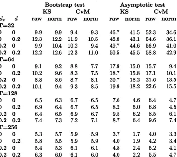
Table 1.1 gives the results of the examination of the level of the bootstrap and asymptotic tests. In this table and in Table 1.2, the heading ’’raw” denotes the size of the test based on the original process 6 (r) defined in (1.4) or (1.6) whereas the heading ’’norm” refers to the size of the test based on the

1 A

levelled process [r (1 — r) ] 2S (r). The bootstrap test is non-conservative, with level approaching the nominal value from above as the sample size increases. Overall, neither KS nor CvM test statistic can be said to generate better test as fax as level is concerned. The actual level tends to be closer to the nominal value when the memory of the error is of short range. Levelling the variance of the process 6 does not seem to bring substantial changes in the size.

The asymptotic test performs poorly for the range of sample sizes under consideration. Again, neither of the Kolmogorov-Smirnov and Cram6r-von

Mises tests dominates the other. Levelling the variance of the process 6 ac­ tually seems to slightly damage the null rejection probabilities for a range of sample sizes.

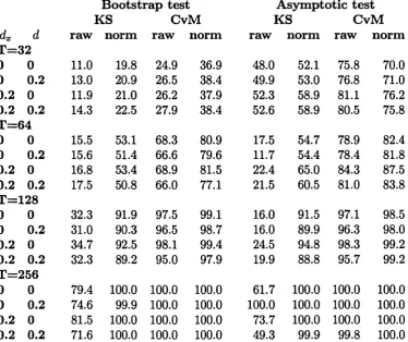
who suspect th at L2-norm CvM test might perform better than sup-norm KS

test in case of the one-time structural break. The rejection probabilities of the asymptotic test are larger than those of the bootstrap test in a majority of parameter combinations. However, such a comparison is not informative since the actual critical values have not been corrected to yield 5% level of the tests. An important observation is th at levelling the variance of the process 6

unambiguously and substantially improves the power of all forms of the test. Overall, the outcome of the simulation exercise provides evidence that the bootstrap procedure proposed in the chapter performs reasonably well already for samples of moderate size. The r