Model Based and Robust Control Techniques for Internal Combustion Engine Throttle Valves

(1)

Model Based and Robust Control

Techniques for Internal Combustion

Engine Throttle Valves

Jacob Lykke Pedersen

A thesis submitted in partial fulfilment of the requirements of the University of East London

for the degree of

Doctor of Philosophy

October 2013

(2)

i

Acknowledgments

I am greatly thankful to my supervisor, Professor Stephen Dodds, whose valuable technical support, knowledge and experience enabled me to finish this work. On a personal level I would like to thank, Professor Stephen Dodds and his wife, Margaret, for the many talks and lunches .

I thank Dr W. Hosny for being my Director of studies since Professor Dodds became Emeritus.

I would also like to thank my colleagues at Delphi for the support and in particular Johan Dufberg for reviewing the work. Also, I would like to take this opportunity to thank my managers, Anthony Potter and Gary Forwards, for supporting this work.

(3)

ii

Summary

The performances of position controllers for a throttle valve used with internal combustion engines of heavy goods vehicles is investigated using different control techniques.

The throttle valve is modelled including the hard stops and static friction (stick-slip friction), which are nonlinear components. This includes a new simple approach to the modelling of static friction. This nonlinear model was validated in the time domain using experimental results, parameterised by experimental data using a Matlab based parameter estimation tool. The resulting state space model was linearised for the purpose of designing various linear model based controllers. This linearised model was validated using experimental data in the frequency domain.

The correct design of each model based controller is first confirmed by simulation using the linear throttle valve model, the specified step response being expected. Then the robustness is assessed in the frequency domain using the Matlab® Control System Design Toolbox and in the time domain by simulation using Monte Carlo based plant parameter mismatching between the simulated real plant and its model used for the control system design. Once satisfactory performance of a specific controller is predicted by simulation using the linear model, this is replaced by the nonlinear model to ascertain any deterioration in performance. Controllers exhibiting satisfactory performance in simulation with the nonlinear plant model are then investigated experimentally.

(4)

iii

controller, observer based robust controller (OBRC) and the polynomial controller. The traditional controllers are designed using partial pole placement with the derived linear plant model. The other controllers have structures permitting full pole placement, of which robust pole placement is an important option. In the pole placement design, the locations of the closed loop poles are determined using the settling time formula.

Despite the use of robust pole placement, the static friction caused a limit cycle, which led to the use of an anti-friction measure known as dither.

The 14 different controllers were investigated for their ability to control the throttle valve position with nonlinear friction, parameter variations and external disturbances. This information was gathered, together with qualitative information regarding ease of design and practicability to form a performance comparison table.

The original contributions emanating from the research programme are as follows:

 The successful application of new control techniques for throttle valves subject to significant static friction

 The first time investigation of partial and robust pole placement for throttle valve servo systems.

(5)

iv

2 MODELLING ... 36

2.1 INTRODUCTION ... 36

2.2 THE ELECTRICAL MODEL ... 39

2.3 MECHANICAL MODEL ... 42

2.3.1Linear Dynamic Model ... 42

2.3.2The Mechanism of Friction ... 47

(6)

v

2.3.4The Friction Model ... 53

2.3.5Hard Stops ... 57

2.4 LINEAR SYSTEM MODEL ... 58

2.4.1State Space Model ... 59

2.4.2Transfer Function ... 61

2.5 NONLINEAR SYSTEM MODEL ... 63

2.6 REDUCED ORDER LINEAR SYSTEM MODEL ... 65

3 MODEL PARAMETERISATION ... 67

3.1 PARAMETER MEASUREMENT ... 68

3.1.1Gear Ratio ... 68

3.1.2DC Motor Voltage Constant ... 68

3.1.3DC Motor Resistance ... 69

3.1.4DC motor inductance ... 69

3.1.5DC Motor Torque Constant ... 69

3.1.6DC motor moment of inertia and the kinetic friction ... 70

3.1.7Throttle Valve System Moment of Inertia ... 74

3.1.8The Coil Spring ... 74

3.1.9Hard Stops ... 76

3.1.10 Throttle Valve System Kinetic Friction ... 76

3.1.11 Static and Coulomb Friction ... 76

3.2 PARAMETER ESTIMATION ... 77

3.2.1Introduction ... 77

(7)

vi

3.2.3Throttle Valve Model Parameters ... 80

3.3 MODEL VERIFICATION IN THE TIME DOMAIN ... 82

3.4 MODEL VALIDATION IN THE FREQUENCY DOMAIN ... 83

4 CONTROL TECHNIQUES AND PERFORMANCE ASSESSMENT ... 88

4.1 INTRODUCTION ... 88

4.2 THE EARLIER DEVELOPMENTS LEADING TO THE PIDCONTROLLER ... 89

4.3 METHODOLOGY ... 91

4.3.1Simulation Details ... 91

4.3.2Experimental Setup ... 92

4.3.3Simulation and Experimental validation ... 95

4.3.4Sensitivity and Robustness Assessment ... 97

4.4 COMMON FEATURES ... 106

4.4.2Pole Placement Design using the Settling Time Formula ... 106

4.4.3Nonlinear Friction and Control Dither ... 113

4.4.4Integrator Anti Windup ... 117

4.5 TRADITIONAL CONTROLLERS ... 120

4.5.2Potential Effects of Zeros ... 122

4.5.3Controller Design ... 125

4.5.4Simulation and Experimental results ... 144

4.6 LINEAR STATE FEEDBACK CONTROL ... 174

(8)

vii

4.6.2State Observer ... 175

4.7 OBSERVER BASED ROBUST CONTROL ... 221

4.7.1Introduction and Brief History ... 221

4.8 POLYNOMIAL CONTROL ... 237

4.8.2Basic Polynomial Controller ... 239

4.8.3Polynomial Control with Additional Integrator for Zero Steady State Error in the Step Response ... 244

4.9 SLIDING MODE CONTROL AND ITS RELATIVES ... 274

4.9.2Basic Sliding Mode Control ... 276

4.9.3Methods for Eliminating or Reducing the Effects of Control Chatter ... 285

5 PERFORMANCE COMPARISONS ... 312

(9)

viii

6.1 OVERALL CONCLUSIONS ... 320

6.1.1Modelling ... 320

6.1.2Control techniques ... 320

6.2 RECOMMENDATIONS FOR FURTHER RESEARCH ... 323

REFERENCES ... 327

APPENDIX ... 331

A.1 ENGINE SYSTEMS OVERVIEW ... 331

A.1.1The Natural Aspirated Diesel Engine ... 331

A.1.2The Turbo Charged Diesel Engine ... 333

A.2 PARAMETERS USED FOR THE SIMULATION ... 341

A.3 CALCULATIONS FOR LINEAR STATE FEEDBACK WITH INTEGRATOR FOR STEADY STATE ERROR ELIMINATION ... 343

A.4 H-BRIDGE WITH OUTPUT CURRENT MEASUREMENT ... 346

A.5 THROTTLE VALVE EXPLODED VIEW ... 348

PUBLISHED WORK ... 349

A COMPARISON OF TWO ROBUST CONTROL TECHNIQUES FOR THROTTLE VALVE CONTROL SUBJECT TO NONLINEAR FRICTION ... 349

(10)

ix

List of Figures

Figure 1.1: An example of a schematic for a turbocharged Euro VI engine

configuration with high pressure EGR and throttle valve ... 24

Figure 1.2: A throttle valve... 26

Figure 1.3: Schematic of a throttle valve ... 27

Figure 1.4: Throttle valve position control system ... 29

Figure 1.5: Desired throttle position demand for a typical drive cycle during DPF regeneration ... 30

Figure 1.6: System settling time definition ... 31

Figure 1.7: Maximum / minimum control effort as function of desired settling time ... 32

Figure 1.8: A section of the generation DPF cycle with different settling times 33 Figure 2.1: A disassembled throttle valve ... 36

Figure 2.2: Throttle valve schematic diagram ... 37

Figure 2.3: Model of a brush DC motor ... 40

Figure 2.4: Electrical schematic of the DC motor ... 41

Figure 2.5: State space representation of equation (2.3) ... 41

Figure 2.6: Throttle body schematic without the DC motor ... 43

Figure 2.7: Gear system ... 43

Figure 2.8: Transfer the moment of inertia and friction to the other side of the gear ... 45

Figure 2.9: Throttle plate side of the gear system ... 45

Figure 2.10: Representation of lumped system ... 47

Figure 2.11: Surface interaction ... 48

Figure 2.12: The same day friction repeatability experiment ... 50

Figure 2.13: Different days friction repeatability experiment ... 51

Figure 2.14: The experiments accumulated differences ... 52

Figure 2.15: Classic friction model (Papadopoulos and Chasparis, 2002) ... 53

(11)

x

Figure 2.17: Friction model implementation... 56

Figure 2.18: New friction model simulation ... 56

Figure 2.19: Hard stop model ... 57

Figure 2.20: Linear throttle model ... 58

Figure 2.21: State variable block diagram ... 59

Figure 2.22: Linear throttle model in control canonical form ... 63

Figure 2.23: Nonlinear throttle model ... 64

Figure 2.24: Second order throttle valve model ... 66

Figure 3.1: Simplified DC motor model ... 70

Figure 3.2: Measured current and the value i T_a

 

... 73

Figure 3.3: DC motor friction and moment of inertia validation ... 74

Figure 3.4: Measure of the coil spring torque ... 75

Figure 3.5: Parameter estimation using the toolbox from Mathworks® ... 78

Figure 3.6: Measurement data used for the DC motor model parameter estimation ... 79

Figure 3.7: Estimation of the DC motor parameters ... 80

Figure 3.8: A subset of the data sets used for the throttle valve model parameter estimation... 81

Figure 3.9: Nonlinear throttle valve model with parameter values ... 81

Figure 3.10: Comparison between the non-linear plant model and the plant (Blue dashed: Experimental data. Green: Simulated data) ... 83

Figure 3.11: An example of a pseudo random binary sequence ... 84

Figure 3.12: Bode plots – Comparison between the non-linear plant model and the plant ... 87

Figure 4.1: Proportional controller applied to the throttle valve... 89

Figure 4.2: Root locus of the system with unity gain feedback control ... 89

Figure 4.3: Step response with proportional controller adjusted for critical damping ... 90

(12)

xi

Figure 4.5: PI controller implemented in dSPACE (simplified diagram) ... 93

Figure 4.6: Experimental hardware ... 95

Figure 4.7: Throttle position demand waveforms for control test ... 96

Figure 4.8: Standard linear control system structure ... 97

Figure 4.9: Sensitivity of the linear throttle valve control loop with a proportional controller ... 100

Figure 4.10: A 2D matrix for parameter variations test ... 101

Figure 4.11: Illustration of 2D parametric variations for Monte-Carlo analysis (Standard deviation = 3 %, Mean value = 0) ... 102

Figure 4.12: Frequency distributions of parameters used for the Monte Carlo analysis (Standard deviation = 3 %, Mean value = 0) ... 103

Figure 4.13: Parameter distribution used for the Monte Carlo (R_a for 



0.01: 0.2



) ... 104

Figure 4.14: Throttle position operation envelope ... 104

Figure 4.15: Settling time definition ... 107

Figure 4.16: Linear high gain robust control system ... 108

Figure 4.17: Root locus with respect to K ... 109

Figure 4.18: Root locus of closed loop system using robust pole placement . 111 Figure 4.19: Block diagrams for ideal step response generation, a) third order, b) fourth order ... 113

Figure 4.20: Dither signal generator ... 114

Figure 4.21: Dither signal level ... 115

Figure 4.22: Experimental result of a P-controller with and without dither ... 116

Figure 4.23: Amplitude spectra ... 117

Figure 4.24: PI controller with integrator anti-windup ... 118

Figure 4.25: Integrator anti-windup performance ... 119

Figure 4.26: The PID controller ... 120

Figure 4.27: The DPI controller with the throttle valve plant ... 121

Figure 4.28: The IPD controller ... 122

(13)

xii

Figure 4.30: Closed loop pole locations for T_s 0.1 [sec] ... 127

Figure 4.31: Closed loop response of a IPD controller with partial pole placement ... 128

Figure 4.32: Throttle valve and IPD controller with differentiation filter ... 128

Figure 4.33: The closed loop poles and zero locations for the IPD controller with a differentiating filter ... 130

Figure 4.34: Simulated step response with/without noise filter compensation 131 Figure 4.35: DPI controller with differentiation filter ... 132

Figure 4.36: The impact of the zero on the closed loop systems response .... 133

Figure 4.37: Closed loop simulation of the DPI controller with a linear throttle valve plant model and limits on the controller output ... 134

Figure 4.38: DPI controller with precompensator ... 135

Figure 4.39: Closed loop simulation of the DPI controller with precompensator cancelling both zeros ... 136

Figure 4.40: DPI controller with integrator anti-windup ... 137

Figure 4.41: Closed loop step response of the DPI controller with integrator anti-windup (Large step) ... 137

Figure 4.42: Closed loop step response of the DPI controller with integrator anti-windup (Small step) ... 138

Figure 4.43: Simplified discrete time DPI controller with feed forward ... 139

Figure 4.44: Simplified continuous time DPI controller ... 140

Figure 4.45: Example of a waveform used for the tuning of the DPI ... 141

Figure 4.46: PID controller with differentiation noise filter ... 142

Figure 4.47: PID controller with differentiation filter, precompensator and integrator anti windup ... 143

Figure 4.48: Closed loop simulation of the PID controller with precompensator cancelling both zeros ... 144

Figure 4.49: Closed loop step response, from 0.2 to 1.3 [rad] ... 145

(14)

xiii

Figure 4.51: The difference between the desired and the experimental closed

loop responses ... 147

Figure 4.52: IPD controller during a spring failure ... 148

Figure 4.53: Maximum / minimum throttle position and DC motor voltage envelope (Standard deviation:  15%) ... 149

Figure 4.54: Control structure used to analyse the sensitivity ... 150

Figure 4.55: IPD sensitivity ... 151

Figure 4.57: Experimental and simulated response of the DPI controller ... 153

Figure 4.58: The difference between the desired and the experimental closed loop responses ... 154

Figure 4.59: DPI controller during a spring failure ... 155

Figure 4.62: DPI sensitivity ... 158

Figure 4.64: Experimental and simulated response of the DPI controller ... 160

Figure 4.66: DPI controller with feed forward during a spring failure ... 162

Figure 4.69: Manually tuned DPI sensitivity... 165

Figure 4.70: PID closed loop step response ... 166

Figure 4.71: Closed loop step response, from 0.2 to 1.3 [rad], using a precompensator ... 167

(15)

xiv

Figure 4.74: PID controller during a spring failure ... 170

Figure 4.77: PID sensitivity ... 173

Figure 4.78: LSF control system ... 174

Figure 4.79: LSF control system with a state observer ... 176

Figure 4.80: A basic third order observer structure ... 179

Figure 4.81: LSF plus integral control ... 180

Figure 4.82: LSF control of the throttle valve with steady state compensation 181 Figure 4.83: The closed loop pole location of the LSF control loop ... 183

Figure 4.84: Pole locations of an LSF plus integral control loop with a robust pole-to-pole ratio of 20 ... 185

Figure 4.85: Observer aided LSF control with integrator for steady state error elimination ... 186

Figure 4.86: Simplified control system block diagram for design of the LSF controller ... 187

Figure 4.87: Third order observer structure ... 188

Figure 4.88: Observer aided LSF with integrator anti-windup used for the experiments and simulations ... 190

Figure 4.89: Throttle valve step response with/without integrator anti-windup (K=0.012) ... 191

Figure 4.90: Restructure a basic observer to a single correction loop ... 192

Figure 4.91: Single correction loop observer with noise filter ... 193

Figure 4.92: Single correction loop observer aided LSF with integrator for steady state compensation ... 193

Figure 4.93: Observer with single loop correction controller ... 194

(16)

xv

Figure 4.95: Experimental and simulated response of the LSF controller with

steady state compensation ... 197

Figure 4.96: The difference between the desired and the experimental closed loop response ... 198

Figure 4.98: Experimental and simulated response of the LSF controller with integrator using robust pole placement ... 200

Figure 4.100: LSF with integrator controller during a spring failure ... 202

Figure 4.101: Simulated closed loop response difference done for a number of different robust pole placement ratios ... 203

Figure 4.104: LSF with integrator sensitivity ... 206

Figure 4.106: Experimental and simulated response of the observer aided LSF controller with integrator using robust pole placement ... 208

Figure 4.108: Observer aided LSF controller during a spring failure ... 210

Figure 4.111: Observer aided LSF control with integral term sensitivity ... 213

(17)

xvi

Figure 4.115: Restructured observer aided LSF with integrator during a spring failure ... 217

Figure 4.118: Restructured observer aided LSF control with integrator sensitivity ... 220

Figure 4.119: Plant and model mismatch ... 221

Figure 4.120: Correction loop controller used for estimating the disturbance U s_e

 

... 222

Figure 4.121: Subtraction of Uˆ_e

 

s from control input to compensate U s_e

 

. ... 222

Figure 4.122: Input conversion block diagram ... 223

Figure 4.123: Overall OBRC structure for a single input, single output plant . 224 Figure 4.124: OBRC structure with a LSF controller ... 225

Figure 4.125: Individual pole placement used for OBRC ... 227

Figure 4.127: Experimental and simulated response of the OBRC ... 231

Figure 4.129: OBRC during a spring failure... 233

Figure 4.132: OBRC sensitivity ... 236

Figure 4.133: a) PID controller converted into the b) basic linear SISO controller form ... 237

(18)

xvii

Figure 4.135: The general structure of the Polynomial control system ... 240 Figure 4.136: Polynomial control of throttle valve with additional integrator ... 244 Figure 4.137: Control system of Figure 4.136 showing controller polynomials246 Figure 4.138: Implementation of the Polynomial control with additional integrator ... 247 Figure 4.139: Closed loop step response with one fast pole ... 248 Figure 4.140: Polynomial control with additional integrator and a second order

plant model used for the controller design ... 251 Figure 4.141: Simulated closed loop response step response at ... 253 Figure 4.142: Simulated closed loop response step response using a

precompensator with the settling time T_sp 



0.2 0.3 0.4



sec ... 254 Figure 4.143: Closed loop step response, from 0.2 to 1.3 [rad] ... 256 Figure 4.144: Experimental and simulated response of the polynomial controller ... 257 Figure 4.145: The difference between the desired and the experimental closed

loop responses ... 258 Figure 4.146: Polynomial controller during a spring failure ... 259 Figure 4.147: Maximum / minimum throttle position and DC motor voltage

envelope at a pole group ratio = 40 (Standard deviation:  14%) ... 260 Figure 4.148: Control structure used to analyse the external disturbance

sensitivity ... 261 Figure 4.149: Polynomial control sensitivity... 261 Figure 4.150: Implementation of the Polynomial control with additional integrator ... 262 Figure 4.151: Closed loop step response, from 0.2 to 1.3 [rad] ... 263 Figure 4.152: Experimental and simulated response of the polynomial controller ... 264 Figure 4.153: The difference between the desired and the experimental closed

(19)

xviii

Figure 4.155: Maximum / minimum throttle position and DC motor voltage

envelope at a pole group ratio = 60 (Standard deviation:  15%) ... 267

Figure 4.156: Control structure used to analyse the external disturbance sensitivity ... 268

Figure 4.157: Polynomial control sensitivity... 268

Figure 4.159: Experimental and simulated response of the polynomial controller ... 270

Figure 4.161: Polynomial controller during a spring failure ... 272

Figure 4.162: Maximum / minimum throttle position and DC motor voltage envelope at a T_s 0.2 sec and a pole group ratio = 16 (Standard deviation:  11%) ... 273

Figure 4.163: A basic variable structure control system ... 274

Figure 4.164: Double integrator plant ... 276

Figure 4.165: Phase portraits for a double integrator plant with b1 ... 277

Figure 4.166: Block diagram of a Bang-Bang controller for a SISO plant ... 278

Figure 4.167: Closed loop phase portrait of a double integrator plant for 1, 2 1 w w  ... 280

Figure 4.168: Closed loop response and bang-bang controller output of a double integrator plant... 280

Figure 4.169: An example of a trajectory for the double integrator plant. ... 281

Figure 4.170: Plant output not directly linked to the plant states ... 282

Figure 4.171: Display of equivalent control for simulation of Figure 4.168. .... 285

Figure 4.172: An example of a basic SMC for a throttle valve plant ... 285

Figure 4.173: Basic sliding mode controller behaviour ... 287

Figure 4.174: Basic SMC with a Control Smoothing Integrator ... 288

(20)

xix

Figure 4.176: Boundary Layer Sliding Mode Control ... 290 Figure 4.177: Switching boundary SMC with measurement noise filtering and

integrator with saturation ... 291 Figure 4.178: Practicable SMC with control smoothing integrator and variable

gain to minimise control chatter for small position errors... 292 Figure 4.179: Boundary layer method SMC with measurement noise filtering 294 Figure 4.180: Boundary layer method SMC with integrator in the forward path

and measurement noise filtering ... 294 Figure 4.181: Closed loop step response, from 0.2 to 1.3 [rad] ... 297 Figure 4.182: Experimental and simulated response of the SMC - control

smoothing integrator method ... 298 Figure 4.183: The difference between the desired and the experimental closed

loop responses with a maximum gain of 700 ... 299 Figure 4.184: The difference between the desired and the experimental closed

loop responses with a fixed gain of 300 ... 300 Figure 4.185: SMC - Control smoothing integrator method during a spring failure ... 301 Figure 4.186: Maximum / minimum throttle position and DC motor voltage

envelope (Standard deviation:  8%) ... 302 Figure 4.187: Structure used for analysing sensitivity ... 303 Figure 4.188: SMC - Control smoothing integrator method sensitivity with a fixed

gain = 700 ... 304 Figure 4.189: SMC - Control smoothing integrator method sensitivity with a fixed

gain = 300 ... 305 Figure 4.190: Closed loop step response, from 0.2 to 1.3 [rad] ... 306 Figure 4.191: Experimental and simulated response of the SMC - Boundary

layer method ... 307 Figure 4.192: The difference between the desired and the experimental closed

(21)

xx

Figure 4.194: Maximum / minimum throttle position and DC motor voltage

envelope (Standard deviation:  15%) ... 310

Figure 4.195: Structure used for analysing sensitivity ... 311

Figure 4.196: SMC - Boundary layer method sensitivity ... 311

Figure 5.1: Step response differences for comparison #1 ... 314

Figure 5.2: Step response differences for comparison #2 ... 315

Figure A: Basic schematic of a natural aspirated Diesel engine ... 331

Figure B: Turbo charger from Cummins Turbo Technologies... 333

Figure C: Basic schematic of a turbo charged Diesel engine ... 334

Figure D: Schematic of a turbo charged Diesel engine with EGR ... 336

Figure E: An example of a schematic for Euro VI engine configuration with high and low pressure EGR ... 338

Figure F: LSF with integrator and plant model... 343

Figure G: H-bridge schematic... 346

Figure H: H-bridge and current measurement boards ... 347

(22)

xxi

List of Symbols

L Inductance [Henry - H]

a

L DC motor armature inductance [Henry - H]

R Resistance [Ohm - Ω]

a

R DC motor armature resistance [Ohm - Ω]

I Current [Ampere - A] V Voltage [Volt]

e

k DC motor voltage constant [V/(rad/sec)]

t

k DC motor torque constant [Nm/A] J Moment of inertia [kg m2_]

x

J Throttle system inertia (lumped)

θ Angle [rad]

ω Angle speed [rad/sec]

spring

k Coiled spring constant [Nm/rad]

N Gear size [m]

r Gear radius [m]

kinetic

k Kinetic (viscos) friction constant [Nm sec/rad]

n System order, if nothing else is stated

s

T Control settling time [sec]

so

T Observer settling time [sec]

 Volume [ 3

m ]

p _{Pressure [} 2

/

N m ] m Mass flow [kg/sec]

Sec Seconds

 

S Switching function

pp

r Pole-to-pole ratio [-]

min pp

r Minimum pole-to-pole ratio [-] h Sampling time interval [sec]

(23)

xxii

s Laplace variable

 Torque [Newton Meter - Nm] Closed loop poles

(24)

xxiii

List of Acronyms

ADC Analogy-to-Digital Converter DAC Digital-to-Analogy Converter DC Direct Current

DPF Diesel Particulate Filter

DPI Derivative Proportional Integral controller e.m.f. Electromotive force

ECU Electronic controller unit EGR Exhaust Gas Recirculation FFT Fast Fourier Transform HGV Heavy Goods Vehicle I/O Input / Output

IPD Integral Proportional Derivative controller

LCR Inductance (L), capacitance (C) and resistance (R) LSF Linear State Feedback

LTI Linear Time Invariant

Matlab® Mathematical tool from Mathworks, Inc. MAXB Micro Auto Box

NOx Nitrogen Oxides

OBRC Observer Based Robust Control

PID Proportional Integral Derivative controller PRBS Pseudo random binary sequence

PWM Pulse Width Modulation SCR Selective Catalytic Reduction

Simulink® Diagram simulation tool from Mathworks, Inc. SISO Single Input – Single Output

SMC Sliding Mode Control

(25)

1. Introduction 24

1

Introduction

1.1 Engine System

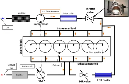
[image:25.595.87.510.259.533.2]

Figure 1.1 shows an overview of the engine system that this research programme supports, a detailed description of which is given in Appendix A.1.

Figure 1.1: An example of a schematic for a turbocharged Euro VI engine configuration with high pressure EGR and throttle valve

The throttle valve, described in more detail in the following section, is the focus of this research programme but this will be equally useful for the other valves employed in the system as each of these has similar characteristics.

Intercooler Air filter

Muffler

En

gi

n

e

b

lo

ck

Fuel injector

Cylinder Turbo shaft

Gas flow direction

Air

Exhaust gas

Intake manifold

Exhaust manifold

EGR valve Throttle

valve

Compressor

(26)

1. Introduction 25

1.2 Throttle Valve

On a petrol engine the throttle valve is used to control the air-to-fuel ratio by applying a variable constraint to the air path, which will reduce the air flow. On Diesel engines (Figure 1.1) the throttle valve is used as a means to increase the EGR rate and reduce the air-to-fuel ratio, in a low power operating range. In this range, the operation of the VGT vanes has no effect and therefore the throttle has to be used. The amount of air into the engine can be controlled by closing the throttle valve, creating a lower pressure in the intake manifold. This lower pressure can also be used to induce more EGR flow through its high pressure path, assuming that the exhaust manifold pressure stays constant.

For the EURO VI regulation, a high EGR_rate is needed in the low power range making use of the throttle valve. During the DPF regeneration, the air-to-fuel ratio needs to be controlled to within a specific range, which will require the use of the throttle valve. Furthermore, the throttle valve can be used to damp engine shaking following key off by closing it.

(27)

1. Introduction 26

1.2.1 Hardware Description

The throttle system (Figure 1.2) consists of a spring loaded throttle plate which is driven by a direct current (DC) motor through a gear system. A pre-windup coil spring applies a residual torque which makes the valve open in the case of an electrical failure. The throttle plate position is measured by a potentiometer type sensor attached to the plate, where fully open = 0 [rad] and fully closed = 1.57 [rad].

Figure 1.2: A throttle valve

The air flow through the throttle valve is a function of the air-to-fuel ratio, EGR rate and after-treatment demands. In the normal operation mode, the throttle reference position is calculated by using the desired throttle air flow, pressures and the temperatures.

The mass flow passing the throttle valve illustrated in Figure 1.3 can be modelled by the isentropic (constant entropy) flow equation for a converging-diverging nozzle (Wallance et al., 1999, Schöppe et al., 2005).

Position sensor

DC motor

Throttle plate

(28)

1. Introduction 27

Figure 1.3: Schematic of a throttle valve For the gas mass flow through the throttle valve:

 

u t

throttle throttle pl

u u

p p

m A C

p R T

  

   _{  }

 _ _ (1.1)

For the non-choked flow (sub-sonic):

1 1

1

2 1

1 ,

1 2

t t t t

u u u u

p p p p

   _  _ _          _   _      _ _{ } _  _ _ _ _ _ _{ } _  _ _     _   _     (1.2)

For the choked flow (sonic):

 1

2 1 1

2 1 , 1 2 t t u u p p p p                    _ _ _ _ _ __ _     

    (1.3)

where

R: Gas constant /

p v

c c

  (1.4 for air)

C: Throttle valve flow coefficient (dimensionless)

throttle

A : Geometrical effective valve area

u

p : Upstream pressure

t

p : Throat pressure

throttle

m : Mass flow through the throttle valve

pl

 : Throttle plate position

The geometrical area for flow passage of an elliptical throttle plate:

p l  t p u p

th ro ttle

m

u

(29)

1. Introduction 28

 

2

 

1

1 cos

throttle pl pl

r

A r

r

  _   _

  (1.4)

where

r: Pipe radius

1

r : Maximum throttle plate radius

In theory, equation (1.1) to (1.4) could be rearranged to get the desired throttle position, using the desired gas flow, the gas temperature and its pressures. In practice, however, it is difficult to get an accurate throttle position by this means due to model parametric errors. This could be circumvented by creating two functions, one based on the physics of the system and a second one based on empirical data, as follows.





1 , , ,

throttle

throttle u u t

u t

u u

m

f m T p p

p p

p R T



    

 _ _

(1.5)









2 1 , , ,

desired

pl f f mthrottle Tu pu pt

  (1.6)

where

2

f : A function which converts the corrected flow f₁ into a throttle position demand

(30)

1. Introduction 29

Figure 1.4: Throttle valve position control system

The torque is proportional to the DC motor armature current. The current is controlled by the throttle valve position controller’s output driver.

1.2.2 Ideal Control System Specification

The aim of the throttle valve position control system design is to achieve the following:

1. The position reference must be followed with a minimum delay and steady state error.

2. The control system must exhibit robustness to minimise the impact of the static (stick-slip) friction, change in friction parameters due to wear & tear.

3. The control system must be able to compensate for failure of the retention spring (pre-windup coil spring).

Figure 1.5 shows an example of a desired throttle valve position demand (0 = fully open, 1.57 = fully closed) for a typical drive cycle during DPF regeneration (source: Delphi Diesel Systems). In the DPF regeneration mode the valve is used to control the narrow air/fuel ratio operation range for the DPF to heat up and stay in the regeneration mode. If the air-to-fuel ratio exceeds the

Throttle valve position controller

Measured throttle position Throttle

position demand

Throttle valve system Armature

(31)

1. Introduction 30

[image:31.595.163.426.180.431.2]

boundaries it can cause the DPF to stop regenerating or in the worst case damage the DPFs ceramic structure due to the generated heat.

Figure 1.5: Desired throttle position demand for a typical drive cycle during DPF regeneration

The dynamics of the desired closed loop system response has to be chosen in such a way that it tracks the demand without too much lag. The lag can cause the air flow to differ from that demanded for significant periods and impact the engine output emission. Choosing too fast a desired closed loop system response can, however, wear down the actuator, in this case the DC motor and gear system in the throttle valve. In addition the speed of response is restricted by the DC motor voltage supply.

Figure 1.6 shows a classic definition of the system settling time T_s (Franklin et al., 2002). This is defined as the time it takes from applying an ideal instantaneous step input to the time at which the systems output has entered

Time [sec]

D

e

s

ir

e

d

t

h

ro

tt

le

p

o

s

it

io

n

d

e

m

a

n

d

[

ra

d

]

0 200 400 600 800 1000 1200 0

(32)

1. Introduction 31

and remained within a specified range of the expected steady state value. In this case the range has been chosen to +/- 5%.

Figure 1.6: System settling time definition

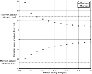
Figure 1.7 shows the minimum and maximum peak values of the controller output during a simulation of a closed loop pulse response (pulse duration 1 second). The simulation is done on a nonlinear throttle valve plant model, with various desired closed loop settling times. The controller is in this case implemented as a state space controller with an integrator in the outer loop to remove the steady state offset. This will be described in more detail in Chapter 4.

The saturation level for the throttle actuator used for this project is +/- 12 volt. Figure 1.7 indicates that peak control effort needed to achieve a desired settling time of 0.1 seconds for a position demand change nearly at the maximum value. This will bring the control system into saturation, but only at the maximum level. The control saturation resulting from attempting to reduce this further would seriously deteriorate the control system performance.

Ts

Steady state value

+/- 5%

(33)

[image:33.595.128.441.137.389.2]

1. Introduction 32

Figure 1.7: Maximum / minimum control effort as function of desired settling time

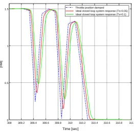
Figure 1.8 is a sample of the desired throttle valve position demand from the DPF regeneration cycle. It shows the simulated impact of the settling time on the system response during the regeneration cycle. When the settling time increases the lag between the desired response (throttle position demand) and the simulated closed loop system response has an increased dynamic lag, as expected.

As stated before, too much lag can cause the emission output level to increase, while controller saturation indicates too fast a response which can prematurely wear the throttle system. The desired closed loop settling time should be chosen as a compromise between lag and saturation of the control system, in this case 0.1 second.

0.08 0.1 0.12 0.14 0.16 0.18 0.2 -15

-10 -5 0 5 10 15 20

C

o

n

tr

o

lle

r

o

u

tp

u

t

a

m

p

lit

u

d

e

l

e

v

e

l

[v

o

lt

]

Desired settling time [sec] Maximum actuator

saturation level

Minimum actuator saturation level

(34)

[image:34.595.165.428.133.391.2]

1. Introduction 33

Figure 1.8: A section of the generation DPF cycle with different settling times

1.2.3 Current Control Techniques

The throttle valve position is currently governed by a PID/DPI controller with feed forward and measures to overcome the static friction. Despite the presence of the integral term, the feed forward is used to counteract the coil spring torque, which also avoids prolonged transient behaviour due to relying solely on the integral action for this. To minimise the effects of the static friction an additional oscillatory signal can be added to the control variable that produces a corresponding torque just sufficient to overcome the static friction. This is known as control dither (Leonard and Krishnaprasad, 1992). The amplitude and frequency of this signal are adjusted at the commissioning stage. This, however, is quite difficult and time consuming.

309 309.2 309.4 309.6 309.8 310 310.2 310.4 310.6 310.8 311 0

0.5 1 1.5

Time [sec]

[r

a

d

]

Ideal closed loop system response (Ts=0.05) Throttle position demand

(35)

1. Introduction 34

In most cases the traditional controllers, i.e., PID/DPI controllers and their variants are employed and tuned by certain procedures, such as Zeigler-Nichols (Meshram and Kanojiya, 2012) or trial and error.

1.3 Motivation

The aim of this research is to study the control techniques used in vehicle power trains for the position control of the throttle valve and to seek new control techniques taking advantage of the flexibility of modern processing technology to achieve an improved performance and reduce the commissioning time. The adoption of model based control techniques and increased robustness against parametric uncertainties and external disturbances are expected to play major roles in reaching this goal.

Model based control system design means the derivation of design formulae for the adjustable parameters of a controller based on a mathematical model of the plant (in this case the throttle valve) and a design specification. Major benefits of this approach are as follows.

a) The control system design can be validated by comparing the response of a simulation of the control system with the expected response set by the design specification.

b) The robustness can be assessed by introducing external disturbances and parametric mismatches in the simulation and observing the resulting deviation of the control system response from the nominal response determined in (a).

(36)

1. Introduction 35

1.4 Contribution

The original contributions emanating from the research programme, that entailed the comparison of fourteen different controllers, are as follows:

 The successful application of new control techniques for throttle valves subject to significant static friction

 The first time investigation of partial and robust pole placement for throttle valve servo systems.

 A simplified static friction model which can be used for other applications.

1.5 Structure of the thesis

(37)

2. Modelling 36

2

Modelling

2.1 Introduction

The throttle system (Figure 2.1) consists of a spring loaded throttle plate which is mechanically connected to a brushed DC motor through a gear system (Scattolini et al., 1997). The pre-stressed coil spring is a safety measure preventing the engine stalling in case of an electric fault, in which the motor is not energised by making the plate go to its open position. The plate’s position is measured by a potentiometer with an output range between 0.5 and 4.5 [V] with total position accuracy of +/- 2%. The non-zero output range is to insure that the control system can detect if the position signal wire breaks.

A pictorial view of the throttle valve components is shown in Figure 2.1. A more detailed exploded view of the throttle valve may be found in appendix A.5.

Figure 2.1: A disassembled throttle valve

The throttle valve system model comprises two parts: an electrical and mechanical model. The electrical model consists of the equations of the

Position sensor DC motor

Tooth wheel with coil spring (inside) Throttle plate

(38)

2. Modelling 37

armature circuit of the DC motor while the mechanical model consists of the equations modelling the mechanical load, including the moment of inertia, the gear system, the spring and friction.

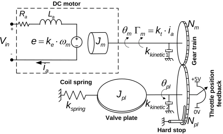
Figure 2.2 shows a schematic diagram of the throttle valve system, starting from the left with DC motor. The DC motor is modelled as an electric load (resistance

a

[image:38.595.108.488.353.582.2]

R and inductance L_a) and back electromotive force (e.m.f.) which depends on the shaft speed. The output torque from the DC motor is proportional to the current. The mechanical system is modelled as a gear system with a moment of inertia and kinetic friction components on both sides. The gear is used to amplify the DC motor torque.

Figure 2.2: Throttle valve schematic diagram

Table 2.1 defines all the parameters of the model.

e m

e



k





+

-DC motor

m



m

J

m

N

pl

N

1

kinetic

k

pl



pl

J

spring

k

Coil spring +5V

0V

T

h

ro

tt

le

p

o

s

it

io

n

fe

e

d

b

a

c

k

2

kinetic

k

Valve plate

G

e

a

r

tr

a

in

Hard stop

a

R

L

_a

in

V

a

i

(39)

[image:39.595.93.511.137.728.2]

2. Modelling 38

Table 2.1: Parameters of throttle valve model

Quantity Description Units

in

V DC motor input voltage V

a

i DC motor armature current A

a

R DC motor armature resistance Ohm

a

L DC motor armature inductance H

t

k DC motor torque constant Nm/A

e

k DC motor voltage constant V/(rad/sec)

e DC motor back e.m.f. generated voltage V

m

 Torque generated by the DC motor Nm

m

 DC motor position rad

m

 DC motor speed rad/sec

pl

 Throttle valve plate position rad

pl

J Moment of inertia for the valve plate kg*m^2

m

J Moment of inertia for the DC motor kg*m^2

spring

k Coiled spring constant Nm/rad

1 kinetic

k The lumped kinetic (viscos) friction constant including the DC motors bearings and half of the gear train friction

Nm sec/rad

2 kinetic

k The lumped kinetic (viscos) friction constant including the throttle plate bearings and half of the gear train friction

Nm sec/rad

m

N DC motor wheel diameter m

pl

N Throttle plate wheel diameter m

/

pl m

(40)

2. Modelling 39

The throttle valve is a butterfly valve type, which means that air flow passing through the throttle valve will not create a load torque and this is therefore not included in the model. The main load torque comes from a linear coiled spring which increases its torque in proportion with the closing angle of the throttle valve.

The mechanical and electrical models of the throttle valve are combined in subsection 2.4 to form a complete linear state space model and the corresponding transfer function model. The linear state space model is used for the controller and observer designs in Chapter 4.

The linear model is extended to form a more comprehensive model in subsection 2.5 that includes hard stops, static and Coulomb friction, making the model nonlinear. The nonlinear model is used to develop the control strategies and to validate them before they are tested on the experimental setup.

In subsection 3 the model is parameterised by using measurements, experiments and a parameter estimation tool from Mathworks®. The parameterised model is then validated in the time and frequency domains.

2.2 The Electrical Model

The DC motor in the throttle valve is mechanically commutated (brushed) with permanent stator magnets (Figure 2.3). The electric current, i_a, which runs through the armature windings, with the resistance R_a and inductance L_a, generates a torque _m equal to the current amplitude multiplied by the constant

t

k

m k it a

(41)

2. Modelling 40

The armature voltage, V_in, supplied by a DC voltage source, drives the armature current, i_a, through the motor. In this case the input voltage source is the throttle valve position controller. The torque is generated by the current through the armature windings interacting with the magnetic field from the stator magnets. The maximum torque is generated when the angle between the conducting windings and magnetic field is 90°. This angle is maintained by the commutator that switches the different sets of armature windings on and off as they rotate under the magnets.

Figure 2.3: Model of a brush DC motor

The torque forces the armature/shaft to spin. The speed of the DC motor, _m , generates a back e.m.f. proportional to the speed via the constant k_e. Thus

e m

ek  (2.2)

The faster the DC motor spins the larger the armature voltage needed to maintain the required armature current, as shown in Figure 2.4.

m

θ

ia

N

S

Brush

Brush Stator magnet

Armature / Rotor windings

Stator magnet

Commutator Bearings

(42)

[image:42.595.207.390.541.645.2]

2. Modelling 41

Figure 2.4: Electrical schematic of the DC motor

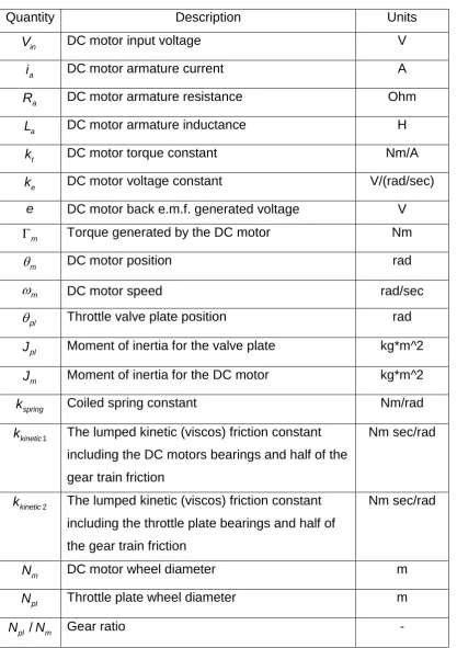
If the DC motor is supplied by a constant voltage, the motor speed will settle to a constant equilibrium value. The armature current will be limited by the back e.m.f. and the resulting electromagnetic torque will be just enough to drive the mechanical friction and load at the constant equilibrium speed. With reference to Figure 2.4, the differential equation modelling the electrical part is as follows.

 

1

 

a m

in a a a e

a m

in a a e

a

dI t d t

V t L R i t k

dt dt

di t d t

V t i t R k

dt L dt



     

 

 _     _

 

(2.3)

The armature current generating the electromagnetic torque, i_a, is found by integrating (2.3). Figure 2.5 shows the state variable block diagram model of the electrical part of the DC motor corresponding to (2.3).

Figure 2.5: State space representation of equation (2.3)

e m

e



K





+

-a

R

L

_a

a

i

in

V

1

a

L

 

in

v s

+

-1

s

 

a

I s

e

k

+ +

a

R

m

(43)

2. Modelling 42

2.3 Mechanical Model

The mechanical model of the throttle valve is split into three sections: the dynamic model, the friction model and the hard stops. The dynamic model comprises the moments of inertia of the mechanical components, the gear train and the friction.

Initially, a linear model will be developed for the model based linear control system design. This includes the kinetic friction, sometimes called the viscous friction, in which the friction torque is directly proportional to the relative velocity between the moving surfaces. A more detailed friction model, however, is needed later, that includes nonlinear friction which is significant in this application. This is developed in subsection 2.3.4, by adding static and Coulomb friction components to the kinetic friction.

Another system nonlinearity consists of the two hard stops of the butterfly valve that limit the movement of the throttle valve plate position. This is modelled using a high gain linear feedback loop approximation explained in subsection 2.3.5.

2.3.1 Linear Dynamic Model

(44)

2. Modelling 43

Figure 2.6: Throttle body schematic without the DC motor

The gear system in the throttle valve consists of three parts (Figure 2.1), a tooth wheel directly mounted on the DC motors shaft, a middle wheel with two different tooth wheel diameters and a tooth wheel mounted on the valve plate shaft. The model, however, is simplified to just two wheels with a single gear ratio as shown in Figure 2.7.

Figure 2.7: Gear system

Here, r_1,2 are the radii of the toothed wheels, _1,2 are the tooth wheel torques and _1,2 are the tooth wheel angles of rotation.

The following relationships hold for this gear system

m 

m



m

J

m

N

p l

N 1

k in e tic

k

p l



s p rin g

k

Coil spring

2

k in e tic

k

p l

J

Valve plate

G

e

a

r

tr

a

in

1





₂ ₂

1



2

r

1

(45)

2. Modelling 44

1 1 2 2

r    r  (2.4)

2 1 2 2

1 2 1 1

N r

 

 _ _ _

 (2.5)

The mechanical model for Figure 2.6 (disregarding the gear train moment of inertia) is based on the following torque balance equation.

, , , , ,

m i m f m i pl f pl sping pl

           (2.6)

where the terms are defined in Table 2.2.

Table 2.2: Torque components of mechanical model

,

i m Jm m

   Torque from the DC motors moment of inertial

, 1

f m kkinectic m

   Kinetic friction torque for the DC motor side

,

i pl Jpl pl

   Torque from valve plate moment of inertial

, 2

f pl kkinectic pl

   Kinetic friction torque for valve plate side

,

sping pl kspring pl

   Spring torque (valve plate side)

(46)

[image:46.595.207.385.122.401.2]

2. Modelling 45

Figure 2.8: Transfer the moment of inertia and friction to the other side of the gear

Figure 2.9 shows a schematic of the plate side of the gear system.

Figure 2.9: Throttle plate side of the gear system

Here, J₂ is the lumped moment of inertia including the valve plate, J_pl, and half of the gear train. On the valve plate side ₂ is the torque acting on the plate shaft from the gear system. The load on this subsystem is the linear spring

2 1

p l

m

N J

N

 

 

 

1

J

m

N

p l

N

1

k in e tic

k

2 1

p l k in e tic

m

N k

N

 

 

 

2





_{p l}

2

J

s p rin g

k

2

(47)

2. Modelling 46

torque which is a function of the valve plate position, the kinetic friction torque and the inertial torque due to the moment of inertia. Thus

2

2 2 2 2

pl pl

kinetic pl spring

d d

J k k

dt dt

 



       (2.7)

The DC motor torque is transferred to the valve plate side by using (2.5). Thus

2

pl m

m

N N

   (2.8)

Then (2.7) can be rewritten as

2

2 2 2

pl pl pl

m kinectic pl spring

m

N d d

J k k

N dt dt

 



       (2.9)

Combining the two parts, i.e., the DC motor part which has been transferred to the valve plate side (Figure 2.8) and the mechanical load represented by equation (2.9), yields

2 2

2 1

pl pl

m x kinetic pl spring

d d

N

J k k

N dt dt

 



       (2.10)

where the lumped moment of inertia is

2

1 2

pl x

m

N

J J J

N

   _ _ 

 

and the lumped kinetic friction is

2

1 2

pl

kinetic kinetic kinetic

m

N

k k k

N

 

 _ _ 

  .

(48)

2. Modelling 47

Figure 2.10: Representation of lumped system

As stated previously, the coil spring is pre-stressed in the factory to keep the throttle open in the case of an electrical failure. To model this, an offset torque is added by means of an angle offset, _{Initial spring}, as follows:





pl pl Initial spring kspring

    (2.11)

It should be noted that this initial spring torque is only to be included in the nonlinear model including the end stops.

2.3.2 The Mechanism of Friction

To move a mechanical part that has close contact with another mechanical part requires a level of force (Figure 2.11). This force level is known as the mechanical friction force. This friction comes from the interaction between the roughness on the two surfaces, where smoother surfaces will decrease the friction force (Popov, 2010).

p l m

m

N





 







p l



x

J

s p rin g

k

k in e tic

(49)

2. Modelling 48

Figure 2.11: Surface interaction

Through time, the throttle valve on a vehicle will be exposed to moisture and dirt that infiltrates the mechanical system. This will result in an increase in the friction between relatively moving components. The amount of friction will change during the day due to temperature change of the mechanical components, but also throughout the lifetime of the throttle valve due to wear. As mentioned before, the friction can cause problems for the controller and even make it limit cycle (Townsend and Salisbury, 1987) (Sanjuan and Hess, 1999) (Radcliffe and Southward, 1990). This points out how important it is to simulate a control system design with a friction model included, prior to implementation.

2.3.3 Preliminary Experiments to Assess the Randomness of the Friction

It would appear from the description in subsection 2.3.2 that the stochastic frictions force is a function of the displacement between the two mechanical surfaces, giving friction force repeatability if the mechanical motion is repeated. Random friction force variations would, however, be produced by quasi-freely moving foreign bodies (dirt). To test the repeatability of the friction effects in the

Moving surface

Fixed surface

(50)

2. Modelling 49

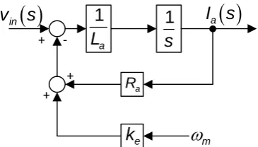
[image:50.595.79.520.439.571.2]

throttle valve application, a set of preliminary experiments was carried out using a standard throttle valve and an existing proportional-integral (PI) position controller with a low amplitude dither. Dither is used as an anti-friction measure which is explained in a later chapter. Essentially good repeatability would indicate that the final control system could be designed to directly compensate for the friction forces. On the other hand, bad repeatability would indicate the need for the final control system to exhibit robustness against unknown friction effects. The system was tested using a ramp function as the position reference input to the controller. A slow ramp is particularly good for testing friction due to its low relative velocity, which exaggerates the effects of static friction, to be explained shortly. The same experiment was repeated firstly four times on one day to detect relatively short term friction variations and then on two different days to detect any longer term friction variations. These experiments are represented in Table 2.3.

Table 2.3: Preliminary friction experiments

Day 1 Day 2

 

pl11 t

 _pl21

 

t

 

pl12 t

 _pl22

 

t

 

pl13 t

 -

 

pl14 t

 -

Note: On day 2 only two experiments were performed.

(51)

[image:51.595.124.482.135.382.2]

2. Modelling 50

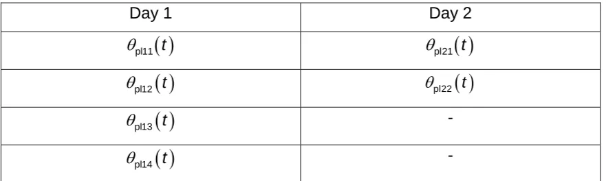
Figure 2.12: The same day friction repeatability experiment

This indicates very little experiment-to-experiment variations (Zoom A-B).

Figure 2.13 shows the superimposed results of two experiments carried out on two separate days.

0 1 2 3 4 5 6 7 8 9 10 0

0.2 0.4 0.6 0.8 1 1.2

Zoom A

Zoom B Zoom B

Time [sec]

T

h

ro

tt

le

p

o

s

it

io

n

[

ra

d

]

 

p l1 1 t



 

p l1 2 t



 

p l1 3 t



 

p l1 4 t

(52)

[image:52.595.127.481.135.381.2]

2. Modelling 51

Figure 2.13: Different days friction repeatability experiment

This indicates more variation than in Figure 2.12. This experiment was repeated with a higher level of dither but this indicated no improvement.

To examine the ensemble variations in errors from one experimental run to the next, i.e., the randomness of the errors, accumulative errors for the above experiments were calculated. These are defined as

 

a , ₀ pl, pl, , 1,2, 1,2,

t

i j i j

e t 



    d j  k  i  j (2.12)

Note that  is the relative time in the sense that data from several data experimental runs, taken at different absolute times, are compared on the same time scale starting at  0. The rationale behind this is that the larger the ensemble variations between experimental run, i, and experimental run, j, the larger the mean slope of e_{a ,}_{i j}

 

t has to be, which must be positive. Only the first two experiments are included here, since four experiments have six associated

0 1 2 3 4 5 6 7 8 9 10

0 0.2 0.4 0.6 0.8 1 1.2

Zoom A Zoom A

Zoom B Zoom B

 

p l 21 t

  

p l 2 2 t



Time [sec]

T

h

ro

tt

le

p

o

s

it

io

n

[

ra

d

(53)

2. Modelling 52

[image:53.595.158.427.175.434.2]

accumulative errors, which are considered sufficient. Figure 2.14 shows the results.

Figure 2.14: The experiments accumulated differences

The figure reflects the observation made by comparing Figure 2.12 with Figure 2.13 that the day-to-day experimental errors are greater than those for experiments performed on the same day. All the graphs of Figure 2.14 indicate considerable ensemble variations from one run to another, in all